Summary

We report on the improvements in EMSolution ver 9.8.2. The improvements are as follows

1. Step input of power supply voltage
2. Periodic repetition of time tables
3. Variable time steps

Explanation

In EMSolution r9.8.1 and earlier, even if the power supply voltage was input as a step change as shown in Fig. 2, the change was interpreted as a dashed line, resulting in inaccurate analysis results. In this section, we discuss the improvements using the model shown in Fig. 1 as an example.

Step input of supply voltage

This model is used and described in "Analysis of a coil connected to a constant-voltage power supply". A voltage source is connected to the coil via a 5 Ohm resistor to excite the central iron core. The magnetic fields in the coil, iron core, and surrounding air are analyzed using the finite element method. Considering symmetry, 1/8 of the total is created and analyzed as a finite element model. The current value flowing in the coil is obtained as a result of the analysis. The voltage source is assumed to be applied stepwise as shown by the solid red line in Fig. 2. When analyzed with the conventional version, the coil current waveform is calculated as shown by the blue dashed line in Fig. 3. The solid black line is the analytical solution, which shows a considerable error. Since the current analysis is a linear analysis, the analytical solution can be easily obtained from the resistance and inductance.
The reason for this error is that in Fig. 2, even if the time variation of the solid red line is input, the calculation uses only the two ends of the step interval and assumes that the voltage of the dashed blue line is added. For this reason, as shown in "Analysis of a coil connected to a constant-voltage power supply", the analysis was performed up to the point before the step change and restarted with that state as the initial value. Now, the voltage step input has been made possible, and this calculation can be performed in a single job; as shown in Fig. 3 with the red line, the results are in good agreement with the analytical solution.

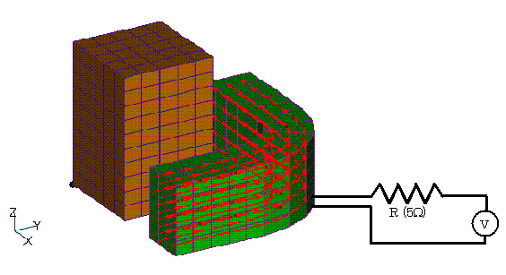
Fig.1 Analysis model

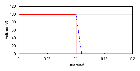
Fig.2 Voltage input waveform

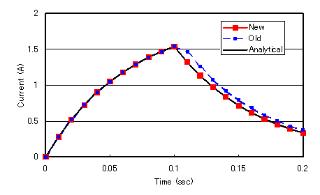
Fig.3 Results of current analysis

Stepwise time changes are entered with different values at the same time in Handbook "input18.2 Time Table". In the case of the analysis example above, it will look like Table1.
For a step change, enter the values before and after the step at the same time. The values before and after the step are linearly interpolated. In the above example, (0.1 0.0) could be set to (0.1001 0.0), for example, but note that this would not be considered a step and the value of 0.1 second would be determined to be 100 $V$, resulting in the same result as the blue dashed line in Fig. 2.

Table.1 Example of Step Input

* TIME_ID * OPTION * 1 4 * NO_TIME_POINTS * 4 * Time(sec) * Value * 0.0 100 0.1 100 0.1 0.0 0.2 0.0

Although unrelated to this additional feature, the case of different NETWORK-THETA values is shown for reference.
For integrals in the time direction, EMSolution allows a q value to be given for the circuit calculation separately from the field calculation. When q=0.5, the difference is the central difference, and when q=1.0, the difference is the backward difference.
As shown in Fig. 4, q=1 (backward difference) reduces accuracy. Note, however, that q=0.5 (central difference) may cause unstable calculations. For the analysis in this document, q=0.5 is fine.

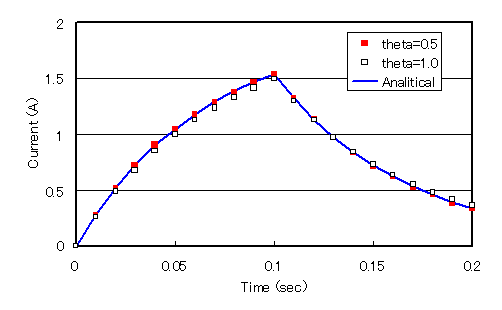
Fig.4 Accuracy of solution for NETWORK-THETA values

Periodic repetition of time tables

With the above additions, multi-step analyses such as the one shown in Fig. 5 can now be calculated in a single job for the same model. At the same time, the time table can be repeated. For other step inputs, only one cycle (in seconds) is required in CYCLE as shown in Table.2. This repetition function can be used not only for step input but also in general.Fig.6 shows the results of current value time variation.

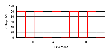
Fig.5 Multi-step voltage input

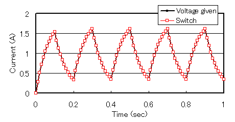
Fig.6 Coil current at multi-step voltage input

Table.2 Example of multi-step input

* TIME_ID * OPTION * 1 1 * NO_TIME_POINTS * CYCLE * 4 0.2 * Time(sec) * Value * 0.0 100 0.1 100 0.1 0.0 0.2 0.0

The above functions can be used with either CIRCUIT or NETWORK in circuit calculations. For NETWORK, a switch function has been added since EMSoluion verr9.8.1, as shown in "Analysis of DC brushless servo motors (using switch function)". The same analysis shown above can be performed by using a switch with a constant voltage source. The voltage source in Fig. 1 can be replaced with the circuit in Fig. 7. The results of this analysis are shown in Fig. 6, with the same results.

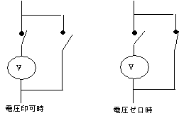
Fig.7 Switching supply voltage by switch

Variable time step

Finally, the most important improvement is the variable analysis time step interval. For example, if a switch is used and the resistance at its opening (Off) is large, the current will change abruptly. In such a case, as shown in the black line in Fig. 8, if the time interval is large, oscillations will appear, resulting in a large error. The analysis in Fig. 8 calculates the case where a switch is inserted in series with the power supply in Fig. 1 and the switch is turned off. The resistance when the switch is off is set to $1k\Omega$. The result of the red line is 1/5 of the calculation time interval between 0.02 seconds after switch Off, and the transient state can be simulated with high accuracy.

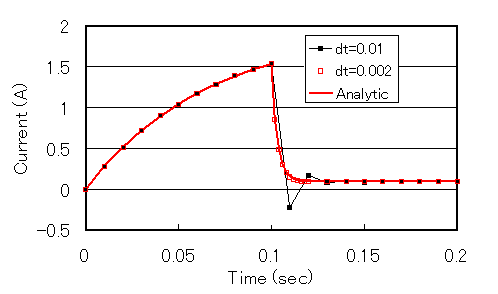
Fig.8 Current time variation during switch

The variable time step input in the example above is shown in Table.3. Change the data in Handbook "input 8. calculation step". The first data is the same as before, but NO_DATA is entered. If this is no input or 1, it is the same as before. Conventional data is calculated at fixed time intervals and does not need to be changed. Then add the number of steps and the time interval. The step numbers in the output are taken in sequence, regardless of the time interval.

Table 3. variable time step input

* NO_STEPS * INITIAL_TIME(s) * DELTA_TIME(s) * NO_DATA * CYCLIC * N_CORRECT * N_BACK * TP_EEC_OPTION * 10 0.0 0.01 3 0 0 0 0 * NO_STEPS * DELTA_TIME(sec) * 10 0.002 9 0.01

This function can be used in general, not only for analysis during switching. It has been requested in the past, and this will reduce the time and effort required to restart the system.
For example, if the step interval after switching is reduced in the analysis of "DC Brushless Servo Motor Analysis (Using Switch Function)", the induced electromotive force waveform shown in Fig. 7 becomes as shown in Fig. 9. The voltage peak at switching becomes sharp and high. However, this calculation assumes that the resistance of the circuit becomes very high due to switching off, so the shorter the calculation time step, the higher the peak value. The peak value itself will not be very meaningful unless a more detailed circuit model is included for the switching current.
In "Electromagnetic field analysis with coupled motion and external circuit system", the plunger motion is analyzed, and a detailed analysis of the behavior when the plunger impacts the wall is shown in Fig. 9. The constant step analysis is sufficiently accurate, but the variable step analysis clearly shows the motion at the time of collision. As shown above, if the computation time step is shortened before and after a sudden change in state, the change in state can be seen in detail. In this case, relatively long computation time steps can be used for other sections, thus saving computation time. Since errors are likely to occur during such sudden changes, shortening the computation time step is effective in improving accuracy. It may also be useful when examining whether the computation time step is sufficient.

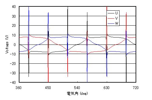
Fig.9 Induced EMF of DC Brushless Motor

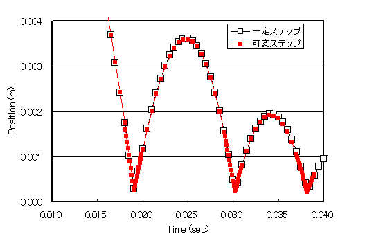
Fig.10 Plunger mover motion