Summary

In general, coupled analysis of electric circuits and finite elements is essential for magnetic field analysis. In EMSolution, three-phase AC power supplies can be coupled with finite elements using the CIRCUIT function and the NETWORK module. This section describes how to model three-phase AC power supplies using the NETWORK module, which allows you to set up electrical circuits more easily and intuitively than CIRCUIT, and explains some points to keep in mind when doing so.

Explanation

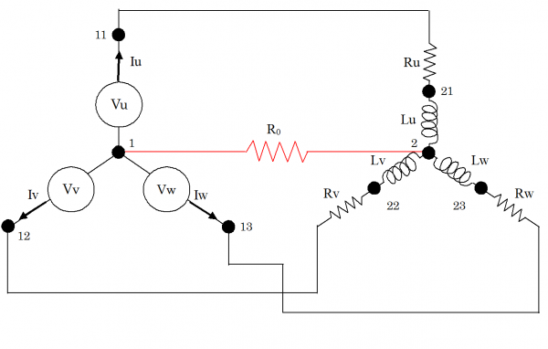
For three-phase AC power supplies ($U$, $V$, $W$), Y-connection (Y-type electromotive force) or $\Delta$-connection ($\Delta$-type electromotive force) is usually the basic method. As the simplest wiring diagram, Fig. 1 shows a Y-connection diagram for both EMF and load current (Y-Y wiring), and Fig. 2 shows a $\Delta$-connection diagram for EMF ($\Delta$-Y wiring). In addition, Fig. 3 shows the Y EMF $\Delta$ load wiring (Y-$\Delta$ wiring) diagram. The same representation is used for either a constant-voltage power supply (VPS in EMSolution) or a constant-current power supply (CPS). On the load side, a resistor R and an inductance $L$ are connected with Y-connection. For simplicity, the load is assumed to be the same in each phase and the power supply is assumed to be balanced. The numbers in the figure indicate the numbers of the nodes in the circuit.

(a)　全体モデル

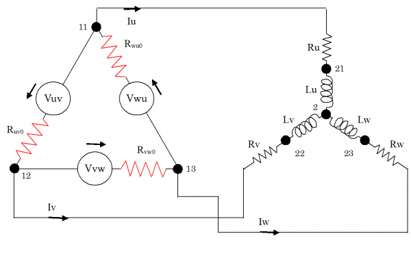
Fig.2 $\Delta$-Y wiring circuit

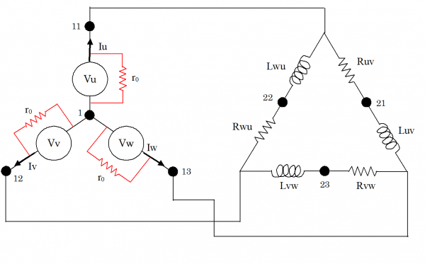
Fig.3 Y-$\Delta$ wiring circuit

First, for the Y-type EMF in Fig. 1, as a precaution, a resistor $R$ must be inserted in the neutral line connecting the neutral points (between nodes 1 and 2) as shown in the figure. In this case, set a resistance value $R_0$ large enough not to affect the results. The current flowing through the neutral point is essentially zero, but if the neutral line is not inserted, the number of independent closed loops will be two, and the three power sources will not be able to operate independently. In the case of a voltage source analysis, the calculation will be performed, but in the case of a current source analysis, the calculation will stop halfway through. Table 1 shows an example of NETWORK data input in EMSolution input data. The load is treated as a constant-voltage power supply, and the load resistance $R$ is set to $1W$ and the inductance $L$ to $0.01H$. $R_0$ is set to $1MW$, which is sufficiently large. Table 2 shows the data of the voltage time variation given to each power supply. The maximum value of current is set to $100V$, and the phases of $U$, $V$, and $W$ are 0°, 120°, and 240°, respectively, and the voltages shown in Fig. 4 are applied. An AC steady-state analysis is performed with a frequency of $50 Hz$, and Fig. 5 shows the time variation of the calculated load current (in this case equal to the supply current).
Next, for the $\Delta$-type EMF in Fig. 2, the input of resistors ($R_{u0}$, $R_{v0}$, and $R_{w0}$) connected in series with the power supply is mandatory. Without inserting these resistors, the resistance of the $\Delta$ loop will be zero. This may cause instability in numerical analysis and large circulating currents may appear in the loop. The resistors in series with the power supply should be small enough. Table 3 shows an example of NETWORK data input. In the Y EMF $\Delta$ load in Fig. 3, in the case of current source (CPS) analysis, the neutral point of the Y EMF must be wired to create an independent closed loop, otherwise it cannot be calculated. Since the CPS is an ideal current source, it can be analyzed by connecting a very large resistor $r_o$ in parallel with the power supply as an internal resistance, just like a real power supply. Table 4 shows an example of NETWORK data input.
Another way to simulate 3-phase AC is to separate the 3 phases and make them independent circuits. In this case, there is no need to insert resistors, but the condition that the sum of the three-phase currents is zero is not satisfied. Alternatively, the circuit can be replaced by an equivalent circuit with two power supplies. In this case, the wiring and phase shift must be properly represented, which is not intuitive to understand or set up. With the NETWORK module, the actual circuit can be input as is in an intuitive manner.
Although equivalent analysis can be performed using CIRCUIT data, it is not easy to understand intuitively because it is necessary to extract independent current variables in advance, examine dependencies between element currents, and input connection matrices and other data into the input data. The NETWORK module can also be used to analyze induction motors by considering the end rings as resistance (see “Handling of Rotor Bars and End Rings in Two-Dimensional Analysis of Squirrel-cage Induction Machines”).

Table 1. Y-Y wiring circuit NETWORK data

* NETWORK * REGION_FACTOR * NETWORK 1 * VPS * ID * NODE1 * NODE2 * TIME_ID * VPS 1 1 11 1 VPS 2 1 12 2 VPS 3 1 13 3 * R * ID * NODE1 * NODE2 * RESISTANCE * R 4 11 21 1.0 R 5 12 22 1.0 R 6 13 23 1.0 * L * ID * NODE1 * NODE2 * INDUCTANCE * L 7 21 2 0.01 L 8 22 2 0.01 L 9 23 2 0.01 * R * ID * NODE1 * NODE2 * RESISTANCE * R 10 1 2 1.0e+006 * END NETWORK * END

Table 2. Time-varying data

* NO_DATA * 3 * TIME_ID * OPTION * 1 2 * AMPLITUDE * TCYCLE(s) * PHASE(deg) * 100 0.02 0.0 * TIME_ID * OPTION * 2 2 * AMPLITUDE * TCYCLE(s) * PHASE(deg) * 100 0.02 -120.0 * TIME_ID * OPTION * 2 3 * AMPLITUDE * TCYCLE(s) * PHASE(deg) * 100 0.02 -240.0

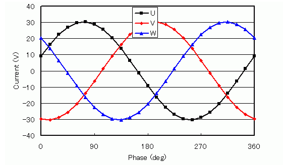
Fig.4 Y-type electromotive force

Fig.5 Y-type load current

Table 3. $\Delta$-Y connection circuit NETWORK data

* NETWORK * REGION_FACTOR * NETWORK 1 * CPS * ID * NODE1 * NODE2 * TIME_ID * CPS 1 11 31 1 CPS 2 11 32 2 CPS 3 11 33 3 * R * ID * NODE1 * NODE2 * RESISTANCE * R 4 11 21 1.0 R 5 12 22 1.0 R 6 13 23 1.0 * L * ID * NODE1 * NODE2 * INDUCTANCE * L 7 21 2 0.01 L 8 22 2 0.01 L 9 23 2 0.01 * R * ID * NODE1 * NODE2 * RESISTANCE * R 11 31 12 1.0e-006 R 12 32 13 1.0e-006 R 13 33 11 1.0e-006 * END NETWORK * END

Table IV. Y-$\Delta$ connection circuit NETWORK data

* NETWORK * REGION_FACTOR * NETWORK 1 * CPS * ID * NODE1 * NODE2 * TIME_ID * CPS 1 1 11 1 CPS 2 1 12 2 CPS 3 1 13 3 * R * ID * NODE1 * NODE2 * RESISTANCE * R 4 11 21 1.0 R 5 12 22 1.0 R 6 13 23 1.0 * L * ID * NODE1 * NODE2 * INDUCTANCE * L 7 21 13 0.01 L 8 22 11 0.01 L 9 23 12 0.01 * R * ID * NODE1 * NODE2 * RESISTANCE * R 11 1 11 1.0e-006 R 12 2 12 1.0e-006 R 13 3 13 1.0e-006 * END NETWORK * END