Electromagnetic field analysis software

Electromagnetic field analysis software
REGION_FACTOR and series and parallel circuits in EMSolution
- TOP >
- Analysis Examples by Functions (List) >
- REGION_FACTOR and series and parallel circuits in EMSolution
Summary
In general, electromagnetic field analysis takes advantage of shape symmetry to create a finite element mesh that is a fraction of the overall model. When a coil is included in the finite element domain, it is connected to an external circuit modeled by CIRCUIT or NETWORK. The circuit can be considered as a whole model or as a sub-model of the finite element domain. In order to ensure that a current of the intended ampere-turn (AT) flows through the coil in the finite element domain, the way the power supply is set up depends on whether the relationship between the circuit (power supply) and the coil is considered as a whole model or a partial model. When setting up a circuit as a whole model, REGION_FACTOR can be used, but the Handbook and other sources may not explain it well enough, so we will explain the relationship between REGION_FACTOR and a circuit, and how to set up a series or parallel circuit with a current source and voltage source.
Explanation
REGION_FACTOR is easy to understand if you think of it as follows.
- If REGION_FACTOR=1, set as a partial model
- If REGION_FACTOR>1, set as series connection=whole model, parallel connection=one parallel sub-model
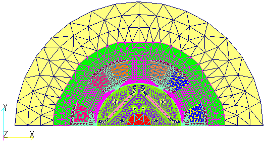
REGION_FACTOR sets the number of times the finite element region is multiplied to matches the circuit. A concrete example is given below. As a simple model, consider a modified version of the IEEJ model with an iron core and coils. Fig. 1(a) shows the overall model and (b) shows a partial model (finite element domain). In the partial model, the X=0 and Y=0 planes are set as $B_n$=0 planes (mirror symmetry plane) and the upper and lower planes as symmetry planes ($H_t$=0), and the coil currents are assumed to flow in the same direction.
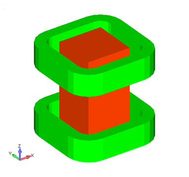
(a) Overall model
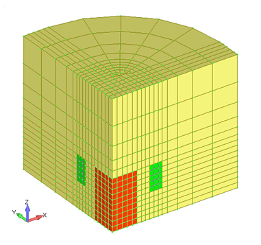
(b) Partial model
(finite element domain)
Fig.1 Iron core and coil model
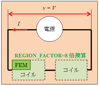
The relationship between the coil and the circuit defined in FEM as ELMCUR is shown in Fig. 2. Fig. 2 (a) is a 2-series circuit and (b) is a 2-parallel circuit. and "FEM" in the coil in the figure represents that 1/4 region of the "coil" is modeled and that four of them are connected in series for symmetry. In other words, the coil defined by the FEM (hereafter referred to as "FEM coil") can be considered as 8 series in (a) and 4 series 2 parallel in (b). The resistance inside the coils is set as conductivity in ELMCUR, so the resistance in the partial model region is calculated and used inside EMSolution. As will be shown later in another example, the coil resistance can also be connected as an external resistance.

(a) 2-serial circuit
(b) 2-parallel circuit
Fig.2 Coil and circuit
For series connection
We assume that the upper and lower coils are connected in series. The current applied will be the same as that of the whole model, even if it is a partial model.
REGION_FACTOR=1
The internal resistance of the coil by ELMCUR is used as the value in the partial model.
-
In the case of current sources Sets the current to be applied to the FEM coil. To do so, set the time function expressing the current to be applied to the current source in CIRCUIT (TYPE=0) or CPS in NETWORK. The voltage (VOLTAGE) and coil flux (FLUX) output in the output file are values in the partial model. Therefore, the voltage and flux can be converted to values in the overall model by multiplying the ratio of the overall model to the partial model = 8.
-
In the case of voltage sources Set the voltage to be applied to the FEM coil. In this case, it is necessary to set the voltage applied to the partial model, so set a time function expressing the voltage to be applied to the voltage source of the CIRCUIT (TYPE=1) or the VPS of the NETWORK. Set the voltage divided by the ratio of the whole model to the partial model = 8. In other words, set the voltage to be applied to the partial model region. The voltage and magnetic flux output to the output file can be converted by multiplying the ratio of the whole model to the partial model = 8.
REGION_FACTOR=8
This will be set as the overall model. This is equivalent to having 8 FEM coils connected in series. The internal resistance of the coil by ELMCUR is multiplied by REGION_FACTOR and used as the value of the overall model.
-
In the case of current sources Set the current to be applied to the FEM coil as in the case of REGION_FACTOR=1. Set a time function representing the current to be applied to the current source in CIRCUIT (TYPE=0) or CPS in NETWORK. The voltage (VOLTAGE) and coil flux (FLUX) output to the output file are multiplied by REGION_FACTOR inside the EMSolution and are values in the overall model.
-
In the case of voltage sources For voltage sources, set the voltage to be applied to the FEM coil. In this case, set the voltage to be applied to the entire model, so set a time function expressing the voltage to be applied to the voltage source of the CIRCUIT (TYPE=1) or the VPS of the NETWORK. The voltage (VOLTAGE) and coil flux (FLUX) output to the output file are multiplied by REGION_FACTOR inside the EMSolution and are the values for the overall model.
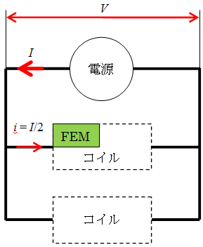
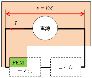
Fig. 3 shows the relationship between the circuit and the FEM coil when REGION_FACTOR=1 and 8 in the case of series connection. When REGION_FACTOR=1, the voltage to the FEM coil is 1/8 of the total voltage, and when REGION_FACTOR=8, the voltage is converted to the whole area.
(a) REGION_FACTOR=1
(b) REGION_FACTOR=8
Fig.3 Relationship between FEM coil and series circuit
Table 1 shows an example of input file settings for CIRCUIT with a $1A$ current source, Table 2 shows the output results with REGION_FACTOR=1 and Table 3 shows the output results with REGION_FACTOR=8. In the case of CIRCUIT, the current and voltage of the power supply are output in "Power Sources" in the output file. In "Sources", the voltage including FEM coil, external resistance and external inductance are output. “Internal resistance" is the internal resistance calculated from the conductivity defined for ELMCUR, and "Internal resistance $\times$ Current" (= voltage) is output as 1/8 of the overall voltage for REGION_FACTOR=1 case and as the overall voltage for REGION_FACTOR=8 case.
Table 1 CIRCUIT data for REGIN_FACTOR=1 or 8 in the case of a current source
Table 2 Output results for REGIN_FACTOR=1 in the case of current source
Table 3 Output results for REGIN_FACTOR=8 in the case of a current source
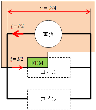
In case of parallel connection
Assume that the upper and lower coils are connected in parallel. For parallel connections, we use the relationship "number of series connections as a circuit (REGION_FACTOR) = ratio of the whole model to the partial-model / number of parallel connections".
REGION_FACTOR=1
In this case, the model is set up as a partial model. The internal resistance of the coil defined by ELMCUR is used as the value in the partial model.
-
In the case of current sources Sets the current to be applied to the FEM coil. To do so, set a time function expressing a current that is 1/2 of the current applied to the whole model to CURRENT SOURCE in CIRCUIT (TYPE=0) or CPS in NETWORK. The voltage (VOLTAGE) and coil flux (FLUX) output in the output file are the values in the partial model. Therefore, to convert the voltage and flux to values in the overall model, simply multiply the factor (=4) obtained by dividing the ratio of the overall model to the partial model (=8) by the number of parallel connections (=2), that is, the number of series connections for one parallel connection.
-
In the case of voltage sources Set the voltage to be applied to the FEM coil. In this case, since the voltage to be applied to the partial model is to be set, set the time function expressing the voltage to be applied to the voltage source in CIRCUIT (TYPE=1) or VPS in NETWORK. At this time, as the voltage value, set the overall voltage divided by the number of series connections in one parallel connection (=4), i.e., the ratio of the overall model to the partial model (=8) divided by the number of parallel connections (=2). The voltage and magnetic flux output in the output file can be converted to values for the overall model by multiplying the coefficient (=4), that is obtained by dividing the ratio of the overall model to the partial model (=8) by the number of parallel connections (=2), that is, the number of series connections for one parallel connection.
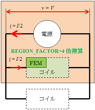
REGION_FACTOR=4
In this case, one parallel connection is considered in the overall model.(See Fig. 4) In other words, it is equivalent to having 4 FEM coils connected in series, which corresponds to 1 parallel connection. The internal resistance of the coil defined by ELMCUR is multiplied by REGION_FACTOR and used as the resistance value for one parallel connection.
- In the case of current sources
Sets the current to be applied to the FEM coil. In this case, set the time function representing 1/2 of the current applied to the whole model to CURRENT_SOURCE in CIRCUIT (TYPE=0) or to CPS in NETWORK. The voltage (VOLTAGE) and coil flux (FLUX) output to the output file are multiplied by REGION_FACTOR in the EMSolution, so they are the values for one parallel connection. The current (= applied current) output in the output file is 1/2 the value of the overall model, so it can be converted to the overall model value by multiplying by 2, the number of parallel connections. - In the case of voltage sources
Set the voltage to be applied to the coil. In this case, set the voltage applied to the overall model. In other words, set the time function expressing the voltage to be applied to the voltage source in CIRCUIT (TYPE=1) or VPS in NETWORK. The voltage (VOLTAGE) and coil flux (FLUX) output to the output file are multiplied by REGION_FACTOR inside the EMSolution and are therefore values for a single parallel connection. The current output in the output file is half the value of the overall model, so it can be converted to the overall model value by multiplying by 2, the number of parallel connections. Fig. 4 shows the relationship between the circuit and the FEM coil when REGION_FACTOR=1 and 4 in the parallel connection case. With REGION_FACTOR=1, the voltage of the FEM coil is 1/4 of the overall voltage, and with REGION_FACTOR=4, the voltage is converted to the overall area, that is equal to the voltage of one parallel connection.
(a) REGION_FACTOR=1
(b) REGION_FACTOR=8
Fig.4 Relationship between FEM coil and parallel circuit
Table 4 shows the output results for REGION_FACTOR=1 and Table 5 shows the output results for REGION_FACTOR=8 for the case where CIRCUIT is used and two parallel connections are made with a 1A current source, i.e. 0.5A is applied to the coil. The voltage is output as 1/4 of the whole model for REGION_FACTOR=1 and as the entire voltage for REGION_FACTOR=4.
Table 4 Output results for REGIN_FACTOR=1 in the case of a current source
Table 5 Output results for REGIN_FACTOR=4 in the case of a current source
As you can see, EMSolution uses REGION_FACTOR to represent a series circuit. However, if there are two or more power supplies with different numbers of series-parallel connections, it is better to set REGION_FACTOR=1, think of it as a partial model, and make settings for each circuit for easier understanding and avoid mistakes.
In the case of parallel connections, even if REGION_FACTOR is used, the current values converted to the overall model could not be input/output. We have created a new option "REGION_PARALLEL" so that current values can be input/output as a whole model even in parallel circuits.
To use this option, set the ratio of the whole model to the partial model as REGION_FACTOR and the number of parallel circuits as REGION_PARALLEL, and the current of the power supply can be input and output as the whole model. In other words, the power supply can be input/output as the whole model, and the coils, external resistors, etc. can be input/output as one parallel value. The default value of REGION_PARALLEL is 1.
REGION_PARALLEL performs the conversion using REGION_FACTOR as explained above inside EMSolution and performs the same calculation as for one parallel. In other words, the current through the coils is given as 1/(the number of parallel connections), and output the power supply as the value of overall model in output file.
In the case of CIRCUIT, the current and voltage values of the overall model are output to "Power Sources" and those of one parallel to "Sources". In the above example, the voltage values are the same in “Power Sources” and "Sources", and the current values in “Sources” are calculated and output as 1/2 of the values in "Power sources". In other words, when setting REGION_PARALLEL, the currents of the power sources are output as values for the entire model, and the currents of the FEM coils, external circuits, etc. are output as values per parallel connection. Table 6 and 7 show an example of using REGION_PARALLEL with CIRCUIT. Table 6 shows the CIRCUIT input data for REGIN_FACTOR=8, REGION_PARALLEL=2 in the case of current source, and Table 7 shows the output results.
Table 6 CIRCUIT data for REGIN_FACTOR=8, REGION_PARALLEL=2 in the case of current source
Table 7 Output results for REGIN_FACTOR=8, REGION_PARALLEL=2, in case of current source
Similarly, NETWORK outputs the current and voltage values of the entire model to CPS or VPS in the output file and those of one parallel to FEM, R, etc. If the coils to be connected in parallel are defined in the finite element mesh (in the above example, an additional mesh is created in the Z direction to make a 1/4 model), set the parallel circuit in the input file directly in NETWORK, etc.
Specific example (D model)
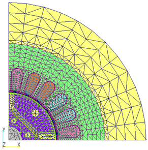
Next, as a concrete example, the D and D1 models, which are the IPMSM benchmark models of the Institute of Electrical Engineers of Japan, will be used. Both the D and D1 models are 4-pole motors with the same size, capacity, etc. The D model is a distributed winding motor with 24 slots and 4 series connections, and the D1 model is a concentrated winding motor with 6 slots and 2 parallel connections, so we will explain how to use REGION_PARALLEL for the D1 model. Fig. 5 shows the two-dimensional finite element mesh for both D and D1 model. The mesh of D model is a one-pole 90-degree model (1/4) and the mesh of D1 model is a two-pole 180-degree model (1/2). In both models, three-phase AC is applied with Y-connection. In the following, the analysis of the no-load induced voltage at the rated speed of 1,500 min-1 (50 Hz) and under the rated current supply condition with a current source by using NETWORK are explained. For reference, a three-dimensional mesh of the D model and an example of a U-phase coil model are shown in Fig. 6 (the coil is modeled using COIL).
(a) D model
(b) D1 model
Fig.5 Two-dimensional finite element mesh
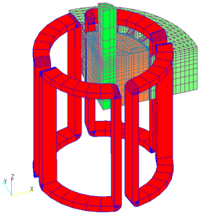
Fig.6 3D model 3D finite element mesh and U-phase coil
D model
The partial model has 6 slots, so 2 slots per phase. The overall model has 24 slots with 4 coils connected in series per phase, so REGION_FACTOR=4. The three-dimensional model shown in Fig. 6 should help you visualize this. In the two-dimensional model, PHICOIL is used for the FEM coils, and two slots per phase are defined as the same PHICOIL. This makes it equivalent to having the coils in the two slots connected in series. The coil resistance is given as an external resistor R, and the value for one phase is set for each phase. Set CPS as the power supply.
1. No-load induced voltage
When the time function ID is set to 0 or the amplitude of the time function ID is set to 0 for CPS, the current is 0A, which is equivalent to opening the circuit for analysis. Transient analysis is required to calculate the induced voltage of the FEM coil. The no-load induced voltage is output to the output file as the value of the whole model with the induced voltage of the partial model multiplied by REGION_FACTOR.
2. Current source analysis under rated current supply condition
For the time function for CPS, set 3-phase AC with an amplitude of 3Arms $\times \sqrt2$, which is the rated current, and a current advance angle of 25 degrees. The voltage in the partial region is multiplied by REGION_FACTOR and output to the output file as the value of the overall model. Note that torque (and iron loss) is output as values of the partial model, so to obtain the overall model value, multiply the partial model value by the ratio of the overall model to the partial model (REGION_FACTOR (4) times for this model). Table 8 shows an example of input file settings under rated current supply conditions with a current source.
Since the current source is Y-connected, it is necessary to set a very large resistance connecting the neutral point. As the UVW current, the amplitude of 3A $\times \sqrt2$ and the phase with a current advance angle of 25 degrees is set. Table 9 shows the resulting outputs. For each of the UVW coils, the voltage (Voltage) and chain flux (Flux) are output, and for the power supply voltage of UVW, the sum of the voltage values produced in the coil and the external resistor is output.
Table 8 NETWORK data for D model (REGIN_FACTOR=4, current source)
Table 9 Output results for D model (REGIN_FACTOR=4, current source)
D1 Model
The partial model has three slots, so there is one slot per phase. Each is set as a U, V and W phase, respectively. The overall model has 6 slots but 2 parallel connections, so REGION_FACTOR=1, based on "the number of series connections as a circuit (REGION_FACTOR) = ratio of the overall model to the partial model / number of parallel connections". Alternatively, REGION_PARALLEL=2 and REGION_FACTOR=2: Ratio of the overall model to the partial model (r10.4.2 or later). This is equivalent to having two FEM coils connected in parallel per phase. Set CPS as the power source.
1. No-load induced voltage
The setting method is the same as for the D model. The no-load induced voltage is output to the output file as the induced voltage of the partial model, that is the induced voltage of the overall model.
2. Current source analysis under rated current supply conditions
If REGION_FACTOR=1, a current of 1/2 of the rated current will flow through the coil, so set a three-phase AC with an amplitude of 1/2 of the rated current (4.4Arms $\times \sqrt2$) and a current advance angle of 20 degrees for the time function for CPS. As in the analysis of the no-load induced voltage, the voltage is output as the value of the overall model and the current through the coil (= 1/2 the current of the overall model) is output to the output file, respectively. When REGIN_FACTOR=2 and REGION_PARALLEL=2, if the time function set in CPS is a three-phase AC with an amplitude of 4.4 Arms $\times \sqrt2$, which is the rated current, and a current advance angle of 20 degrees, the FEM coil is analyzed as if 1/2 of the rated current flows through it. As in the analysis of the no-load induced voltage, the overall model value is output as the voltage, the set rated current value as the CPS current value, and the current value of 1/2 of the rated current value as the FEM and R current values are output to the output file.
Torque (and iron loss) is output as a value of the partial model, so please multiply the ratio of the part
Torque (and iron loss) is output as a value of the partial model, so please multiply the ratio of the partial model to the overall model by 2 to convert it to the overall model value. Table 10 shows an example of input file setting under the rated current supply condition by current source. As with the D model, the Y-connection is used, so a very large resistance is set up connecting the neutral point. For each phase of UVW, current of 4.4A $\times \sqrt2$ as current amplitude and 20° phase as current advance angle is input. Table 11 shows the output to the output file. The current for one parallel is output as the current for the coil and external resistors, and the total current is output to the power supply.
Table 10 NETWORK data for D1 model (REGIN_FACTOR=4, current source)
Table 11 Output results for D1 model (REGIN_FACTOR=4, current source)
When performing a three-dimensional analysis, both the D and D1 models are axial 1/2 models (see Fig. 6 for the D model). This is because the embedded magnet is a single piece in the axial direction. Since it is axially one-half model, the coils can be considered to be connected in series for both the D and D1 models. Therefore, REGION_FACTOR=4×2=8 for the D model and REGION_FACTOR=2, REGION_PARALLEL=1 or REGION_FACTOR=4, REGION_PARALLEL=2 for the D1 model (since r10.4.2).
Thus, when setting up FEM coils in a finite element mesh, series and parallel connections of the coils can be represented by considering the ratio of the overall model to the partial model and how many parallel connections there are.
In case of COIL (external current magnetic field source)
For COIL, which is an external magnetic field source, modeling is created as a whole model, but the relationship to the circuit must be considered in the finite element mesh domain, since it cannot be set up using model symmetry. As an example, let us model the iron core and coil model shown in Fig. 1 using COIL. Fig. 7 shows the finite element mesh and COIL. The coil resistance is input as an external resistance.
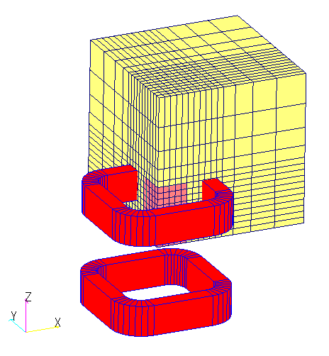
Fig.7 Iron core and coil model defined by using COIL
In the case of series connection, it can be considered as in the case of ELMCUR. For the coil resistance, input the value of the partial model when REGION_FACTOR=1 and the value of the overall model when REGION_FACTOR=8.
In the case of parallel connection, COILs cannot be connected separately in series, as the schematic shows. This is because COILs are not considered outside the symmetry plane of the mesh. In this example, only the FEM region is considered for the magnetic flux chained to the COIL. Therefore, the magnetic flux chained to the COIL below the symmetry plane of the mesh is zero. Therefore, two COILs are connected in series as 1 series, and parallel connection is considered with REGION_FACTOR.
Parallel connection of COIL
The upper and lower coils are connected in parallel, but COIL can be either 1 series or connected in series in a circuit. In order to make sense of parallel connections, we use the same relationship as in ELMCUR: "number of series connections as a circuit (REGION_FACTOR) = the ratio of the whole model to the partial model / number of parallel connections".
1. When REGION_FACTOR=1
The model is set as a partial model. Enter the value of the coil resistance as an external resistance in the partial model.
2. When REGION_FACTOR=4
The model is to be set up as one parallel out of the overall model. In the case of COIL, the parallel connection is considered in REGION_FACTOR. For the coil resistance, input the value multiplied by REGION_FACTOR, i.e., one parallel value, as an external resistance.
3. When REGION_FACTOR=8 and REGION_PARALLEL=2
As mentioned above, the power supply is treated as the whole model and the other parts as one parallel part. The coil resistors are input as external resistors, with the value multiplied by REGION_FACTOR, i.e., the value for one parallel.
In this way, parallel connections can be made even if the COIL is located beyond the symmetry plane of the mesh. Note that in transformers, when coils are connected in parallel, in order to simulate secondary resistance, the value of the secondary resistance must be converted to one parallel value before inputting it.
How to use
As mentioned above, setting REGION_PARALLEL eliminates the need to convert REGION_FACTOR according to series or parallel circuits or to convert currents to values in parallel in setting inputs or interpreting outputs. Also, the output value in the output file does not need to be converted to a parallel connection, and it is possible to check whether or not a parallel connection is made based on the relationship between the power supply and the current flowing through the coil.
Also, it is not necessary to convert the parallel connection in the output output output, and it is possible to check whether the parallel connection is made based on the relationship between the power supply and the current flowing in the coil. This function can be used for both CIRCUIT and NETWORK, and can be used for all current and voltage sources in STATIC, AC, and TRANSIENT analysis.
This function can be used for both CIRCUIT and NETWORK, and can be used for all current and voltage sources in STATIC, AC, and TRANSIENT analysis. The ratio of the partial model to the whole model is set as REGION_FACTOR, and the number of parallels is set as REGION_PARALLEL. The default value of REGION_PARALLEL is 1. In the analysis results, the overall current value is output for the power supply, and the current value for one parallel is output for elements other than the power supply.
For CIRCUIT
For NETWORK
Download
Iron Core and Coil Model (ELMCUR):
- REGION_FACTOR=4
- input_2blockCoils_r4.ems
- REGION_FACTOR=8,REGION_PARALLEL=2
- input_2blockCoils_r8p2.ems
- Mesh Data:
- o Using static magnetic field analysis with ELMCUR
Iron Core and Coil Model (COIL):
- REGION_FACTOR=4
- input_2blockCoils_r4.ems
- REGION_FACTOR=8,REGION_PARALLEL=2
- input_2blockCoils_r8p2.ems
- • Mesh Data:
- mesh file required
D Model:
- Static magnetic field analysis for initial values:
- input2D_static3A25deg.ems
- Transient analysis:
- input2D_transient3A25deg.ems
- Mesh Data:
- pre_geom2D.neu
- rotor_mesh2D.neu
D1 Model:
- REGION_FACTOR=1:
- For initial value : input2D_static4.4A20deg.ems
- Transient analysis : input2D_transient4.4A20deg.ems
- REGION_FACTOR=4,REGION_PARALLEL=4:
- For initial values : input2D_static4.4A20deg_p2.ems
- Transient analysis : input2D_transient4.4A20deg_p2.ems
- • Mesh data : pre_geom2D.neu,rotor_mesh2D.neu
Analysis Examples by Functions
Coupled with external circuit system
- Example of Periodic Current Change Input of Constant-current Power Supply
- NETWORK and CIRCUIT settings in a three-phase circuit
- Transformer Analysis
- Improvement of Power Supply Input Method
- Time-dependent variable resistance elements
- Y-connection and $\Delta$-connection
- NETWORK Nonlinear Element Table Entry
- REGION_FACTOR and series and parallel circuits in EMSolution
- Coupled analysis with MATLAB/Simulink
- 鎖交磁束ベースのモータビヘイビアモデル
©2020 Science Solutions International Laboratory, Inc.
All Rights reserved.