Summary

Electromagnetic devices such as IPM motors are often created using MATLAB/Simulink (Mathworks Inc.), a multi-domain simulation and dynamic system for control circuit systems that also include power electronics, which can simulate circuits more similar to actual devices. It is considered to be highly versatile in that it can simulate circuits that are more similar to actual devices.　EMSolution and MATLAB/Simulink (MATLAB 7.10.0 R2010a) can be directly coupled for analysis.　This module can be used in the same way as the coupled analysis module with PSIM, and allows direct coupling of electrical and control circuits, including power electronics, with FEM for analysis.

Explanation

１．Introduction

EMSolution has the capability of coupling electromagnetic field analysis with external circuit systems and equations of motion on its own.　However, it is not powerful enough to simulate complex control circuits such as motors, so we have developed and already released a coupled analysis module with PSIM that can also simulate power electronics. On the other hand, electromagnetic devices such as IPM motors are often created using MATLAB/Simulink (Mathworks Inc.), a multi-domain simulation and dynamic system for control circuit systems that also include power electronics, which can simulate circuits more similar to actual devices. It is considered to be highly versatile in that it can simulate circuits that are more similar to actual devices.　We are pleased to report that EMSolution and MATLAB/Simulink (MATLAB 7.10.0 R2010a) can now be directly coupled for analysis.　This module can be used in the same way as the coupled analysis module with PSIM, and allows direct coupling of electrical and control circuits, including power electronics, with FEM for analysis.

2. Coupled analysis method

MATLAB/Simulink provides a variety of modules, but here we show an example of coupled analysis between Simulink and SimPowerSystems, an electric circuit module that also includes power electronics.　Basically, the method is the same as the coupled analysis with PSIM, and the execution module of EMSolution uses the DLL (Dynamic Link Library).　Since EMSolution is modularized as an S-Function in Simulink, the Electric Value of SimPowerSystems cannot be passed on as is, but must be converted to a Physical Value in Simulink before being passed on. Therefore, the Electric Value of SimPowerSystems cannot be passed on as-is.　 Therefore, not only SimPowerSystems but also other power electronics software that can perform coupled analysis with Simulink can be used in the same way.

2.1.1 Coupled Electric Circuit Systems

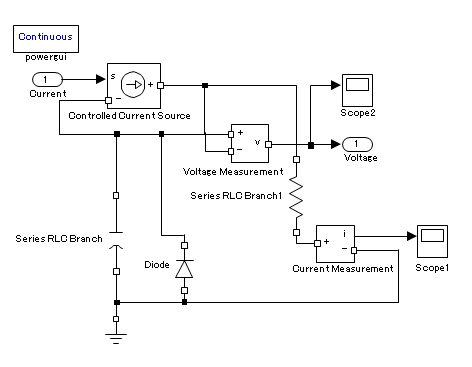
EMSolution alone has a coupled analysis function with electric circuit systems. As in the coupled analysis with PSIM, the voltage calculated in Simulink is input to EMSolution, which performs electromagnetic field analysis, obtains the current of the voltage source, outputs it to Simlink, and performs stepwise calculations. As in PSIM, in Simulink, the voltage source of EMSolution is the Controlled Current Source of SimPowerSystems, and the voltage at both ends of the source is obtained by Voltage Measurement and passed to EMSolution.

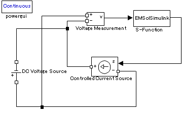
Fig. 1 Coupled electric circuit system

The settings on the EMSolution side are the same as for PSIM, with OPTION=4 for the time function to be given to the the NETWORK module’s voltage source: VPS.

The Simulation Type in Simulink is set to Continuous. The solver in Simulink has variable steps, but EMSolution can only handle fixed steps, so the solver in Simulink should also be a fixed step solver. The fixed step (basic sample time) is set to "auto" by default, but in this case, the minimum time step of the circuit element is detected and calculated. Therefore, if the sample time for elements other than EMSolution is set to "-1: Inheritance", Simulink automatically selects the time step set in EMSolution as the fixed step for coupled analysis with EMSolution. Simulink automatically selects and analyzes the time step set in EMSolution as a fixed step. Of course, it is possible to explicitly set a time step to the fixed step, but depending on the Simulink element used, it may not be possible to set a fixed step that differs from the EMSolution.
Fixed step solvers will be discussed in the analysis examples.

2.2 Coupled equations of motion

EMSolution also has a function to analyze the coupled equations of motion, but it is better to use Simulink when complex operations for position and velocity are involved. Simulink also provides differential and integral elements, making circuit creation intuitive.
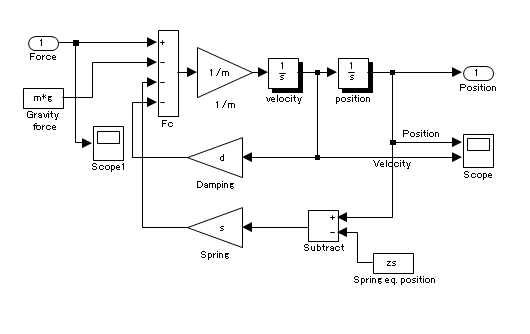
Consider the following equation of motion:

$$m\ddot{z}+d\dot{z}+s(z-z_s)=F-mg $$ $$\ddot{z} : acceleration, \dot{z} : velocity, z : position置$$

where $m$, $g$, $s$, $z_s$ and $d$ are the mass, gravitational acceleration, spring coefficient, spring equilibrium position, and damper coefficient, respectively.

Equation (1) can be expressed as a circuit in Simulink as shown in Fig.2. The acceleration is integrated by the integrating element to obtain the velocity and position. F is the external force, which in this case represents electromagnetic force. In this way, the equations of motion can be described by Simulink and coupled with EMSolution. As with PSIM, the settings are the same as for the Dynamic module, and the IDs for passing values to and from the external software are set.

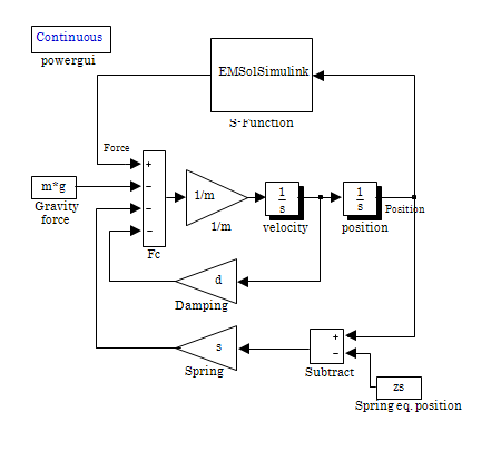
Fig.2 Coupled equations of motion

3. Example of analysis

3.1 Plunger model

The analysis of the plunger model shown in Fig. 3 is coupled with Simulink. Both the electrical circuit and equations of motion are described and analyzed in Simulink.

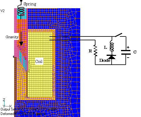
Fig.3 Plunger model

(i) Overall view

(ii) Electrical circuit subsystem

(iii) Equation of motion subsystem

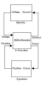
Fig.4 MATLAB/Simulink plunger model

The electrical circuit and equation of motion circuit portions shown in Figs. 1 and 2 are represented as a subsystem. The electrical circuit is shown with the FEM mesh in Fig. 3. The electrical circuit receives voltage from the electrical circuit subsystem and returns current. From the equation of motion subsystem, we receive the position and return the electromagnetic force. EMSolution can define diode element as a function, but here we will use the diode element provided in Simulink. The coil is connected in series with the diode, but the diode includes the inductance of the coil in the electric circuit subsystem. EMSolution takes the voltage from the electric circuit subsystem and returns the current value obtained by coupling with the FEM.

The Equation of Motion Subsystem receives the position and returns the electromagnetic force calculated by the FEM. The fixed step is set to "auto" and the analysis is performed with the same time step dt=1.e-4sec as EMSolution. The initial voltage of the capacitance is set to 50 V to prevent the plunger from colliding with the bottom surface. The time integration on the EMSolution side is set to the defaults THETA=2/3, THETA_NETWORK=0.5, and THETA_MOTION=0.5.

Figures 5 and 6 show the plunger position and current variation in the circuit for EMSolution, PSIM coupled, and Simulink coupled. The Simulink coupled analysis is performed using the fixed step solver with ode1: 1st-order Euler method, ode3: 3rd-order Euler method, and ode5: Dormand-Prince method. The diode elements are also available in PSIM, so there is a slight difference from EMSolution, but they fit well together. The deviation from EMSolution and PSIM is rather large for the Simulink ode1: 1st-order Euler method, and it seems that a higher-order step solver than the ode3: 3rd-order Euler method should be used to obtain accurate results.

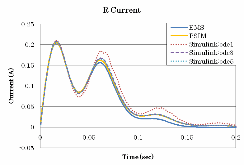
Fig.5 Resistor Current

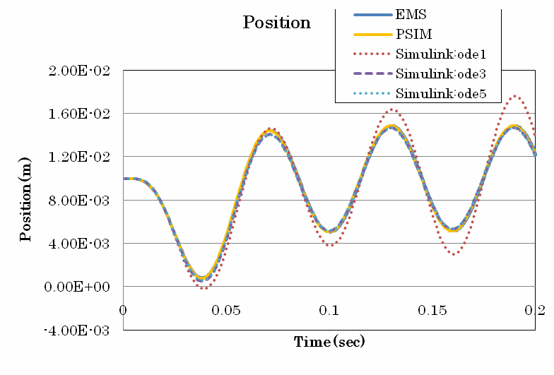
Fig.6 Plunger position

3.2 Analysis of Brushless Servo Motor

The model is adapted from the example PWM inverter-controlled model provided in Simulink, with the SPM motor element part replaced by EMSolution. The SPM motor is used here. The number of poles, capacity, command speed, direction of rotation, direction of external load, etc. are also different from the motor model in the Simulink example, and are changed accordingly. The motor also has a friction coefficient that depends on the rotational speed. EMSolution receives three-phase coil voltage and external load torque from Simulink as inputs and outputs three-phase coil current, rotation speed, rotation position, and torque. The PWM inverter uses a hysteresis comparator method to feed back the rotation speed, which is used as a PI (proportional-integral) signal to control the q-axis current. A rotational speed command value of $314 rad/sec$ ($=18,000deg/sec$) is given and analyzed with zero external torque (no load) at startup, and an external torque of 4$Nm$ is given in steps at 0.03s of startup. The PWM inverter type can be changed to a PWM transport wave comparison method. The motor is three-phase Y-connected, but in Simulink, representing the Y-connection as it is would result in an error. Therefore, the motor is changed to two-phase wiring with line-to-line voltage and then changed back to three-phase voltage and connected to EMSolution (because once the two currents in the y-connection are determined, the remaining current are determined by the sum of them). It is probably no problem to connect directly to EMSolution without Y-connection on the Simulink side. PWM inverter and dq-abc conversion are also described as blocks in Simulink.

The contents have not been changed from the Simulink example, so we omit the explanation. For the time integration on the EMSolution side, THETA and THETA_MOTION are set the same as in the Plunger model, and THETA_NETWORK=1: backward difference is more stable, so it is set as such. The fixed step solver in Simulink is set as ode3: 3rd-order Euler method, which was found to be accurate enough. For the analysis, the time step of EMSolution is set to 1.e-4 sec, Simulink is set to 1.e-5 sec as fixed step analysis, and 500 steps are analyzed up to 0.05s with different values for the time step of EMSolution and Simulink.

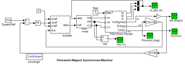
Fig.7 PWM inverter SPM motor model

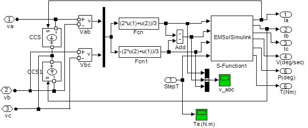
Fig.8 EMSolution Simulink three-phase Y-connection model

Figures 9 to 13 show coil phase voltage, line voltage, coil current, rotational speed, and torque. The speed gradually increases from startup, reaching the command speed in approximately 0.008s. Although this is no-load operation, the average torque is slightly greater than zero because of the friction coefficient that depends on the speed. When load torque is applied at 0.03s, the voltage changes accordingly, and the current and torque increase, but it can be seen that the speed quickly returns to a speed close to the command value.

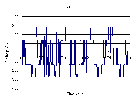
Fig.9 U-phase voltage

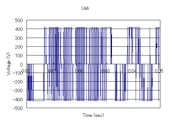
Fig.10 UV phase voltage

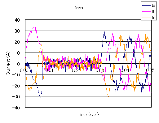
Fig.11 Coil current

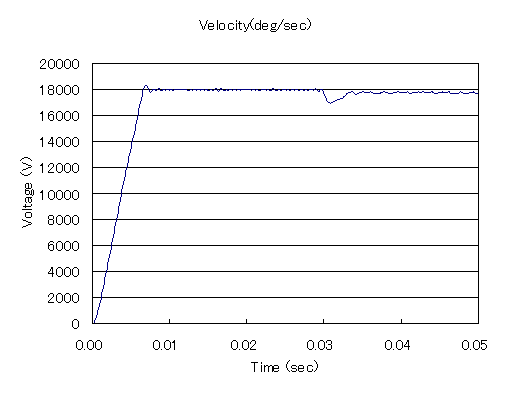
Fig.12 Rotation speed

Fig.13 Torque

4. Conclusion

This report describes the magnetic field analysis in conjunction with MATLAB/Simulink, which can be coupled with Simulink to calculate the electric circuit, equations of motion, and power electronics control circuit simultaneously. The results obtained by EMSolution alone and in coupled analysis with PSIM are in good agreement with each other, indicating that this method is valid. On the other hand, Simulink’s functions are so abundant that they cannot be introduced in this analysis, but we believe we have shown the method of coupled analysis with EMSolution. The following is an example of a case in point. Although the model used in this report is a two-dimensional model and not very realistic, we hope you can see some of the advantages of this method.

Note that EMSolution must also be run on Windows, as it is currently (2011/01/24) running on Windows only. The coupled analysis requires the MATLAB/Simulink module and the EMSolution DLL MATLAB/Simulink version. If you would like to use EMSolution on a Linux system, please contact us.

How to use

To use, start MATLAB/Simulink and set EMSolution DLL MATLAB/Simulink version as S-Function. The extension of the DLL for coupled analysis was .dll before MATLAB 7.0.4 (R14SP2), but since R14SP3, it is .mexw32 for 32bit/.mexw64 for 64bit. The setting method of the EMSolution input file is exactly the same as that for coupled analysis with PSIM, so please refer to that. For coupled analysis with Simulink, place the EMSolution DLL MATLAB/Simulink version in the same folder as the Simulink configuration file.mdl, EMSolution input file, and mesh file. The Network module is required for coupling with electric circuits, and the Dynamic module is required for coupling with equations of motion.

Download

Plunger electric circuit

• Complete set of motion Simulink model data

PWM inverter brushless servo motor

• Simulink model data set