Summary

Here is a simple example of an electromagnetic field analysis that couples with motion and an external circuit system. Consider a plunger model as shown in Fig. 1.

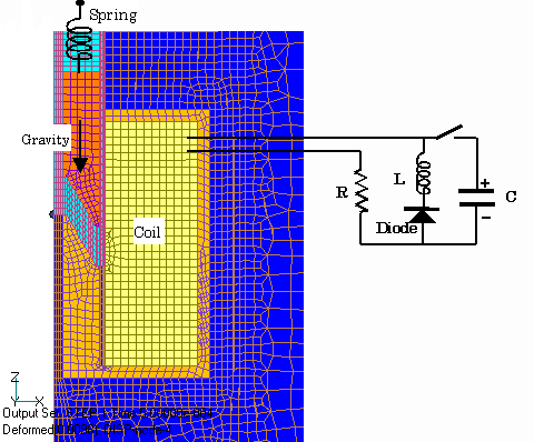
Fig.1 Plunger analysis model

Explanation

The analysis is assumed to be two-dimensional axisymmetric. Spring, gravity, and electromagnetic forces act on the mover. The coil is assumed to be connected to an external circuit as shown in Fig. 1. The external circuit consists of a capacitor, a resistor, an inductance and a nonlinear element (diode). Initially, the capacitor is charged, and the switch is closed to start the discharge. After the capacitor has discharged, current flows into the diode. The stator and mover of the plunger are nonlinear magnetic materials with high electrical resistance. Fig. 2 shows the motion and the time variation of the eddy current density distribution. Since the resistivity of the magnetic material is quite large, the eddy current density is low and no skin effect is observed.

Fig.2 Motion of mover and eddy current density distribution ($A/m^2$)

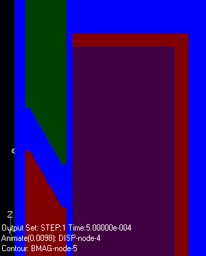
Fig.3 Variation of magnetic flux

The vertical position variation of the mover is shown in Fig. 4. The spring force and gravity are balanced at the initial position of 10 mm, then the coil is excited and an electromagnetic attractive force acts to initiate the downward motion. It bounces back with a reflection coefficient of 0.7 at Z=0.2mm. After several collisions, it stops at Z=0.2mm. As the coil current decreases, the electromagnetic attractive force weakens, and the mover is pulled back upward by the spring force, repeating simple harmonic oscillations. The frictional force is not included here.

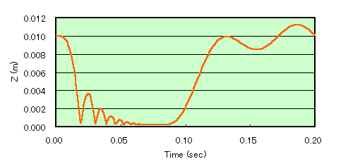
Fig.4 Variation of vertical position of mover

The current variations in the capacitor, diode, and coil in the circuit are shown in Fig. 5. First, a discharge from the capacitor causes a current to flow into the coil. The oscillation caused by the collision of the mover causes a current change in the coil that is synchronized with the oscillation. When the capacitor discharge ends and the voltage reverses, current flows into the diode, and current continues to flow in the coil.

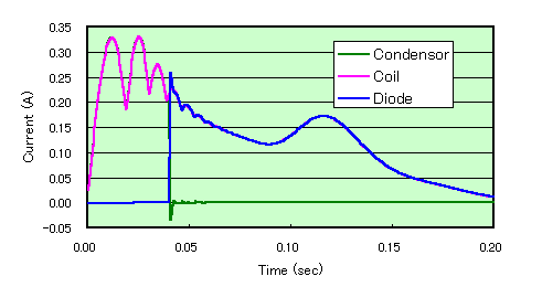
Fig.5 Current variation in the circuit

Fig. 6 shows the variation of the electromagnetic force acting on the mover. Note that in the current calculation, the spring constant is 1 N/mm and the gravity is 0.882 N. There is not much variation in the electromagnetic force due to mover vibration. This can be attributed to the fact that when the position of the mover changes, current flows through the coil that conserves magnetic flux, and the magnetic flux between the poles does not fluctuate much.

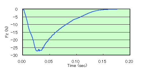
Fig.6 Change in electromagnetic force acting on mover

Although the above analysis is simple and not very realistic, I believe it shows an interesting phenomenon that can only be solved by coupling the motion and the external circuit system. It is expected to be applied to actual design and analysis in the future. For analyses involving motion such as the present calculation, deformation of the finite element mesh is necessary. In this calculation, the mesh in the air region (light blue area) in Fig. 1 is deformed to handle the motion. The mesh at both ends of the motion is input, and the mesh is automatically generated internally at each time. In this case, for simplicity, a two-dimensional analysis is shown, but general three-dimensional problems can be handled in the same way. Rotational motion can also be analyzed in the same way. The coupled equations of motion can also be applied when using the sliding method, and motors and generators can also be analyzed and solved by coupling their motions. For external circuits, resistors, inductances, capacitors, and nonlinear elements such as diodes can be handled.
Previously, connection matrices were input, and the power supply was connected to the finite element circuit. Now, the above elements, including finite element circuits, are connected to circuit nodes, making the input intuitive and easy to understand. Although the coupling of motion and external circuit systems may increase the computation time, the computation time for conventional electromagnetic fields is dominant, and the increase in computation time due to the coupling is not significant. In the calculation above, 400 steps were calculated in 678 seconds (DEC a 433 MHz).