Summary

In EMSolution, for analyses in which the distance between the poles changes, such as an electromagnetic plunger, the analysis is performed by deforming the elements in the air region around the mover (armature).

Explanation

The method of requiring two mesh data (pre_geom and deform_mesh) to interpolate the nodal positions of the deformed air region during deformation motion is shown in "Plunger Motion Analysis (Electromagnetic Field Analysis Coupled with Motion and External Circuits)". The method of enclosing the deformation region with control elements (Control Volume elements) and automatically deforming it inside EMSolution is shown in "Improvement of Deformation Motion Function". In a two-dimensional analysis, nodes at the maximum deformation position can be created as deform_mesh, although this is more time-consuming, but in a three-dimensional analysis, the method of specifying the deformation region with control elements is more suitable. For linear actuators with large strokes, if there are no poles on the stationary side (stator) in the direction of motion of the moving side (mover), it would be better to use the sliding method described in "Motor Analysis" in the same way as for a linear motor. Here we show an example of analysis using a three-dimensional model in which the distance between the poles changes and control elements are used.
To perform an analysis involving deformation, the Deform module is required for deformation motion, and the Motion module is required for the sliding method.

Plunger type electromagnet

The two-dimensional analysis of a plunger-type electromagnet is shown in "Electromagnetic Field Analysis with Coupled Motion and External Circuit" and "Improvement of Deformation Motion". Fig. 1 shows the analytical model. The model is borrowed from Reference [1]. The analysis domain is a quarter model due to the symmetry of the model. The magnetic path is closed by the yoke core on the lower side of the model, and since it is expected that there is little magnetic flux leakage, the air region on that side is not created very far away.

Since magnetic flux leakage is expected on the upper and lateral sides, an air region is created slightly outward from the lower side. The control elements are made of triangular prisms and hexahedral finite elements, which share a node and must have at least one node touching the moving side and stationary sides, respectively. However, the deformation domain elements do not have to be created within a single control element; they can be calculated if they are created within the domain of control elements. (For example, if there are two control elements, there is no need to create a deformation domain element that takes their boundaries into account; it is sufficient to have a deformation domain element within the two control elements, meaning that there can be a deformation domain element that spans between the control elements.) The approximate dimensions are given in Reference (1), but the material properties and calculation conditions are not, so we assume that the mover (plunger) and yoke core are made of S45C with nonlinear magnetic properties, and that an excitation current of 10 A flows through 100 turns of the coil. The coils are defined by using ELMCUR, giving a turn density ($T/m^2$) to the CURRENT. It would be easier to understand if we set the number of turns T for the coil, give a current A at CIRCUIT or NETWORK, which is the power supply, and consider that a current of ampere-turns (AT) flows through the coil.

ELMCUR can be used when the mesh division is layered in the circumferential direction and the element cross-sectional area is constant. ELMCUR can be used only for hexahedral and triangular prismatic elements, with the above restrictions. Therefore, ELMCUR cannot be used if you want to divide a coil mesh in tetrahedral form or if it is difficult to divide the coil mesh in layers. In such cases, please use SDEFCOIL or PHICOIL.

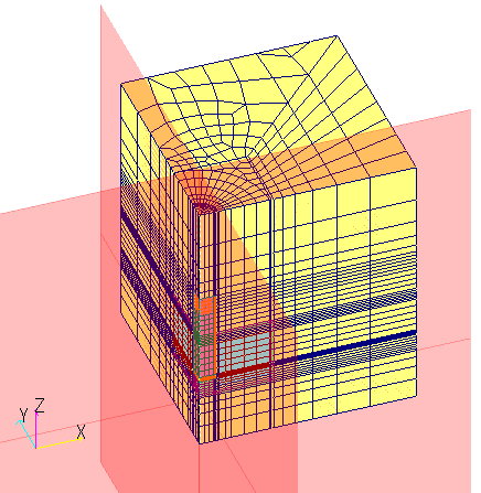
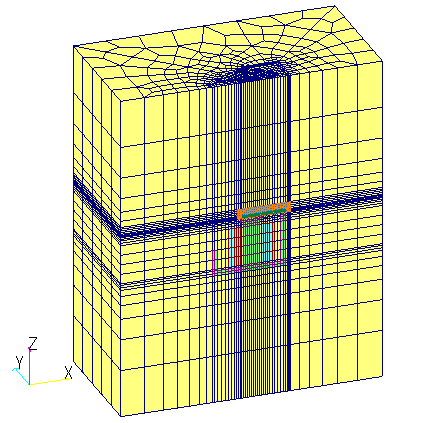
(i) Analysis mesh

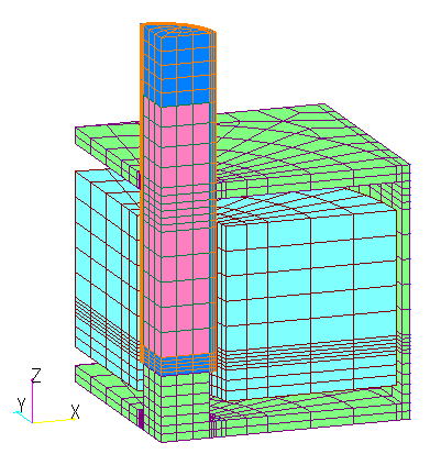
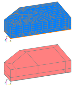
(ii) Deformation air region around the fixed part and mover
(red surfaces represent symmetry planes)

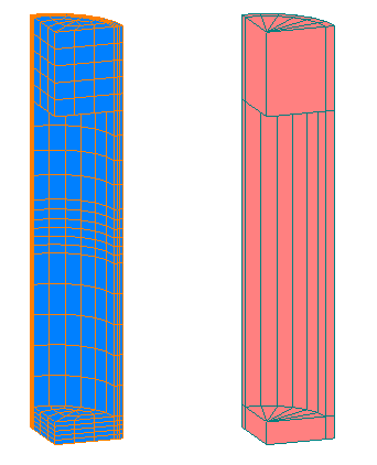
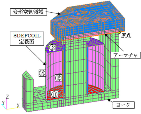
(iii) Deformed air region and control elements
(Control Volume)

Fig.1 Plunger-type electromagnet analysis mesh

Let us try to obtain the steady-state attractive force characteristics under the above conditions. The analysis is performed by forcing the gap distance between the plunger and the lower magnetic pole of the yoke to move from 1 mm to 6 mm. The analysis is a static magnetic field analysis, but it can be set up and analyzed in the same way when eddy currents are included as forced motion or when there are time-dependent elements in the circuit system.

First, define the reference position. POSITION 0 sets the relative position (distance) of the pre_geom mesh from the reference position. The mesh creation position at the bottom of the plunger is 3 mm above the magnetic poles. If we determine this 3 mm above the magnetic pole as the reference position, we set POSITION 0 = 0 m, and, since we want POSITION 1 to be 0.2 mm from the magnetic pole, we set POSITION 1 = -0.0028 m as the relative position from the reference position. Therefore, the relative position from the reference position is set to the time function as time series data. In this case, 1mm above the magnetic pole is -0.002m, and 3mm is 0m. The Deform, which defines the deformation motion, is set to motion in the Z direction. If you want to use the top of the magnetic pole (0mm) as the reference position, then POSITION 0 = 0.003m, since it is relative to the reference position, and POSITION 1 = 0.0008m, since POSITION 1 is relative to POSITION 0. In this case, 1mm from the magnetic pole is 1mm, and 3mm above the magnetic pole is 3mm, which may be easier to understand. The idea is to set POSITION 0 and POSITION 1 to relative positions (distances) from an appropriately determined reference position. As long as POSITION 1 – POSITION 0 are the same value, the result will be the same no matter how they are set.

Fig. 2 shows the steady-state attractive force Fz analyzed by setting the distance from the yoke pole to the plunger from 1 mm to 6 mm in 1 mm increments. The electromagnetic force increases rapidly when the plunger is close to the magnetic poles, and conversely decreases when the plunger is further away. The characteristic is close to linear as it moves away. This is because the mover is subject to two forces: the electromagnetic force between the poles (magnet-pull) and the electromagnetic force between the magnetic flux leaking from the mover through the coil to the yoke and the coil current (solenoid-pull), and the magnet-pull and solenoid-pull are affected by the penetration depth of the mover into the coil [1]. A magnetic flux density vector diagram for a distance of 1 mm from the magnetic pole to the plunger is shown in Fig. 3.

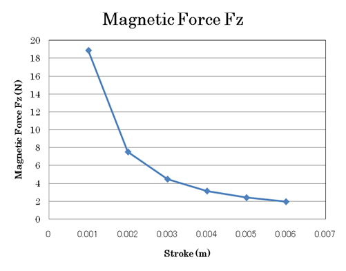
Fig.2 Steady-state absorption characteristics
(Plunger type electromagnet)

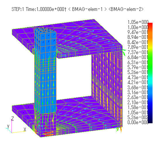
Fig.3 Magnetic flux density vector distribution diagram
(Plunger type electromagnet)

Hinged Electromagnetic Relays

Next, a hinged electromagnetic relay is shown. This is known as a typical dc electromagnet that allows rotational motion with a narrow angle. The analytical mesh is shown in Fig. 4. The finite element mesh is created in the 1/2 region cut in the ZX plane from symmetry. The upper mover core is designed to rotate when it is attracted by the magnetic poles in the coil with the hinge (fulcrum) on the yoke as its center of rotation. The armature is not in contact with the yoke and has a gap of 0.1 mm. Material properties and calculation conditions are not listed in the literature (1) for this model either, so the mover (armature) and yoke core are given the nonlinear magnetic properties of S45C. Since the electromagnetic relay is subjected to a sudden application of voltage, it is assumed that there is a coil resistance large enough to prevent excessive current flow, or that a load resistor is connected. Since neither the coil resistance nor the load resistance is known, we will assume a rated current of 200 mA and a rated voltage of 12 V, although slightly larger than the literature values, and determine the external resistance to be 60 Ω, including the coil resistance. The number of coil turns is set to 1000T so that the steady-state attractive force (torque) is approximately 0.05Nm when the gap length between the mover and the magnetic poles is 0.2mm. The coil is rectangular, and SDEFCOIL is used to set up the coil by specifying four sides. Let us calculate the steady-state attractive force characteristics under the above conditions, including by way of confirmation. Perform a static magnetic field analysis by forcibly moving the gap distance between the armature and the upper magnetic poles of the yoke from 0.1 mm to 0.7 mm. As in the above example, we want to deform the mesh, so we set the Deform parameters. Since the mesh is created at a distance of 0.1mm between the armature and the yoke poles, the angle is set to 0deg. We will use this as the reference position. Since the rotation axis is assumed to be the Z-axis in EMSolution, the Y-axis of the global coordinates is defined as the Z-axis of the local coordinates. Note that the local coordinates can be defined at any position, but the output values are output as global coordinate values, in which case a coordinate transformation is required. Since this is a rotational motion, set the angle to POSITION 1 and POSITION 2: POSITION1=0deg, POSITION2=45deg. For the time function, set the relative angle from the reference position in degrees (deg).

(i) Analysis mesh
ZX plane: Symmetry plane

(ii) Deformation air region around the fixed part and the mover

(iii) Deformed air region and control elements (Control Volume)

Fig.4 Analysis mesh of hinged electromagnetic relays

Fig. 5 shows the steady-state attractive force (torque) analyzed with a gap distance between the armature and the upper yoke poles ranging from 0.1 mm to 0.7 mm in 0.1 mm increments. Since the analysis results are output as a global coordinate system, the armature torque is My(Nm). This shows that an electromagnetic attractive force of about 5 Nm is obtained with a gap length of 0.2 mm, as intended. Fig. 6 shows the magnetic flux density distribution for gap lengths of 0.1 mm and 0.7 mm.

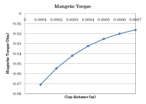
Fig.5 Steady-state attractive force of hinged electromagnetic relay

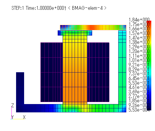
(i) Gap distance 0.1mm

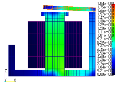
(ii) Gap distance 0.7mm

Fig.6 Magnetic flux density distribution of hinged electromagnetic relay under steady-state attractive force [T]

Next, the operating characteristics of the electromagnetic relay are simulated. We analyze the transient motion characteristics up to the position where the armature comes into contact with the yoke poles when voltage is applied in a pulsed manner. For this purpose, it is necessary to analyze the coupled equations of motion of the rotation including the electromagnetic force, the spring supporting the armature, and the gravity due to its own weight. These conditions are given in the Dynamic module.

The equation of motion due to the spring and gravity is given by Equation (1). The moment of inertia and gravity are defined in rotational coordinates and given to MASS and CONST_FORCE, respectively. The spring equilibrium position is set at a gap distance of 0.7 mm, the spring constant SPRING_CONST is set to switch at 5 ms after voltage is applied, and the initial position at that time is calculated using formula (1) and given to INITIAL The initial position at that time was calculated from formula (1) and given to INITIAL_POSITION.

$$T_g + T_k = l \cdot g / r – k ( x – x_0 ) 　　　　　(1)$$

$T_g$ : Torque due to gravity($Nm$),
$T_k$ : Torque due to spring($Nm$),
$I$ : Moment of inertia (inertia) ($kg・m^2$),
$g$ : Gravitational acceleration -9.8$m/ s^2$,
$r$ : Armature length($m$),
$k$ : Spring constant($Nm/deg$),
$x_0$ : Spring equilibrium position($deg$),
$x$ :Displacement (initial position) ($deg$)

With this setup, EMSolution can perform a coupled analysis with the equation of motion for rotation given equation (1) as an external force. The results are output to a motion file. The switching point is assumed to be at a gap distance of 0.1mm, and this position is set as the lower limit LOWER_LIMIT=0deg. The time step is set to 0.25ms and the voltage is set to 0V at -0.25ms, one step before, to simulate a pulse of 12V applied at 0s for analysis.

Generally, the armature and yoke of an electromagnetic relay are considered to be assembled after machining the parts and then subjected to strain relief annealing. It is known that processing and annealing degrade magnetic properties and conductivity. Therefore, we will also analyze the armature and yoke considering eddy currents with a conductivity of 2.0e+6S/m and compare the results with those neglecting conductivity. The analysis results are shown in Fig. 7 for the coil current, Fig. 8 for the torque, and Fig. 9 for the gap distance. From these results, it is possible to simulate the phenomenon that the excitation current temporarily decreases as the armature is attracted into the magnetic pole yoke due to the increase in inductance. When conductivity is given, the operation is delayed due to eddy currents caused by the pulsed voltage applied. If conductivity is ignored, the armature position is gradually attracted, and at 5 ms it is closest to 0.1 mm, the switching point, and after a slight bounce it comes to rest. When conductivity is taken into account, the switching point is reached slightly later than 6 ms. Similarly, the torque also shows that the pull force is different with and without conductivity. In both cases, the torque reaches a constant value a little after the armature comes to rest. Fig. 10 shows the magnetic flux density distribution with and without conductivity. In the case without conductivity, the magnetic flux density is almost uniformly excited in the iron core, whereas in the case with conductivity, the magnetic flux density is concentrated on the surface of the iron core due to the skin effect, resulting in a lower pull force. From the above, it seems necessary to pay attention to whether or not eddy currents are taken into account in order to simulate the characteristics of the actual machine.

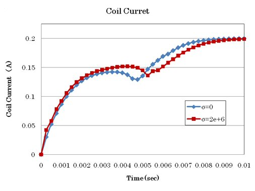
Fig.7 Coil current waveform (Hinged electromagnetic relay)

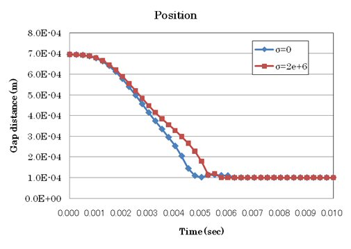
Fig.8 Gap distance (Hinged electromagnetic relay)

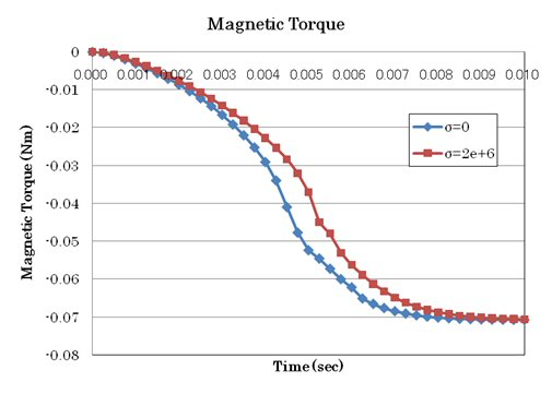
Fig.9 Operating attractive force (Hinged electromagnetic relay)

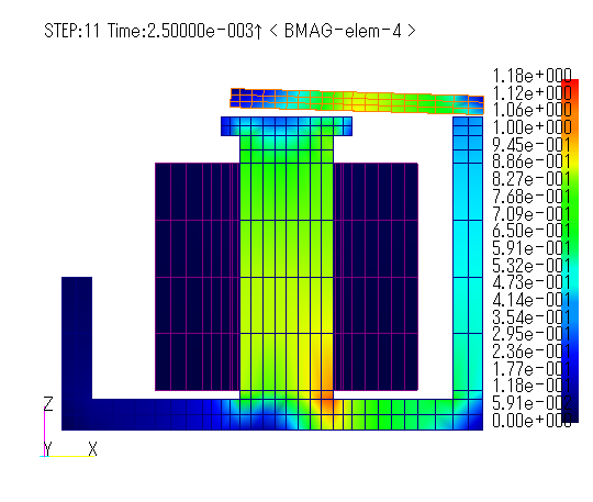
(i) No conductivity

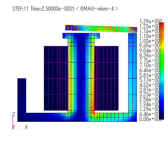
(ii) With conductivity

Fig.10 Magnetic flux density distribution with and without conductivity at hinged electromagnetic relay t=2.5ms

Conclusion

From the above, we believe we have shown how plunger and hinged electromagnets can be analyzed using EMSolution’s Deform and Dynamic modules. Although the deformation region must be air, we hope we have shown that it is relatively easy to set up even a three-dimensional model by using control elements. Although we only used DC operation in this analysis, I believe that it is also possible to analyze AC electromagnetic contactors that operate in the same way with AC. We hope this will be a useful reference for your use.

References

[1] Kawase, Ito: "Practical Analysis of Electric and Electronic Equipment", Morikita Publishing Co.