Summary

EMSolution provides two types of current field sources: one assumes wound coils and the other assumes bulk conductors. Current field sources that assume wound coils ("ELMCUR", "SDEFCOIL", and "COIL") assume that the current distribution across the coil cross-section will be or is uniform. In contrast, bulk conductors have current distribution depending on their geometry and eddy currents under AC magnetic fields. "PHICOIL" and "SUFCUR" are available as magnetic field sources for bulk conductors. In this section, we will explain how to analyze bulk conductors in direct current (DC) using PHICOIL and SUFCUR, and how to analyze them in steady state with a small amount of alternating current (AC) as a disturbance superimposed on the DC.

Explanation

A simple example shown in Fig. 1 is used to illustrate this. Assume two-dimensional axisymmetry, with a ring of conductor plates in the ZX plane and current flowing in the circumferential direction. Also, the top of the mesh is assumed to be $B_n=0$. This is equivalent to having a conductor plate on the upper side with mirror symmetry and current flowing in the opposite direction.

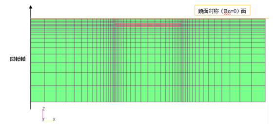
Fig.1 IEEJ Benchmark Model (D model)

First, a DC analysis is performed. The DC analysis can be performed with static magnetic field analysis (STATIC). A current source analysis is performed with DC current = 3000A. The current distribution in the bulk conductor plate is determined by the geometry, so the use of PHICOIL is appropriate. In the case of this model, the analysis is axisymmetric, so the current distribution in the conductor cross-section is inward (Fig. 2). Note that PHICOIL does not output the eddy current loss of the conductor to an output file. To calculate eddy current loss, set the conductivity in PHICOIL, EMSolution calculates the resistance of the conductor section and outputs it to the output file, so use that resistance and current to calculate the eddy current loss using I²R. In this model, the value is 0.01069W. The resistance output to the output file is multiplied by REGION_FACTOR. REGION_FACTOR=1 is used here to make it easier to compare with eddy current losses using SUFCUR.

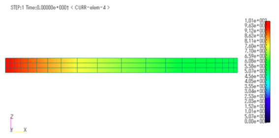
Fig.2 Current distribution in a conductor cross-section
(DC analysis using PHICOIL)

◆output of output file

**** Phi_coil resistance (calculated from conductance ) of source series ID 1 is 1.18773e-009 ****

Next, let’s try to use SUFCUR for DC analysis. However, SUFCUR cannot be applied to STATIC due to its functionality, so a transient analysis (TRANSIENT) must be performed. In the case of TRANSIENT, a numerical transient state occurs at the beginning of the analysis even when DC current is applied, so it is necessary to analyze until it settles (becomes steady). Here, the time increment is set to 50 ms and 800 steps (40 s) are analyzed.

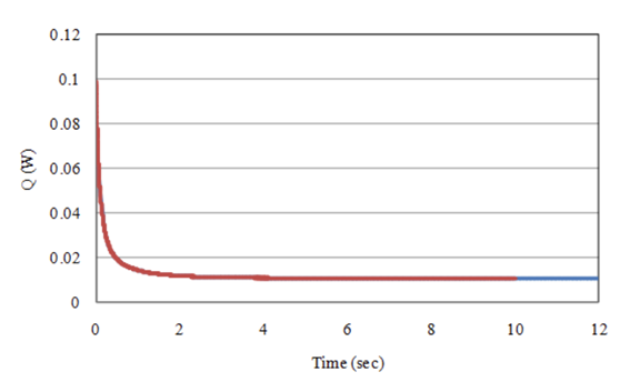
Fig. 3 shows an eddy current loss graph. It can be seen that the numerical transient state that occurred at the beginning of the calculation is gradually decreasing and approaching steady state. When the graph is enlarged, it can be seen that it becomes steady after about 25s. This is because eddy currents are generated by the DC current applied on the step in the early stage of the calculation, and the time constant of the eddy currents brings it close to the steady state. Fig. 4 shows the eddy current distribution in the conductor cross section. In the initial stage of the calculation, the current is closer to the surface of the conductor due to the eddy currents, but at steady state, the distribution is the same as that of PHICOIL. Naturally, the obtained eddy current loss is 0.01069W, which agrees with the PHICOIL result. Note that the eddy current loss obtained by using SUFCUR is output to an output file and is only for the mesh region.

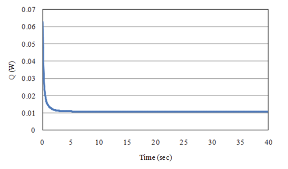
(a) Overall

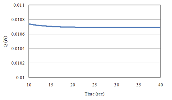
(b) Enlargement

Fig.3 Eddy current loss graph (DC analysis using SUFCUR)

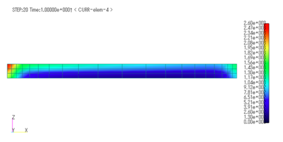
(a) Initial calculation

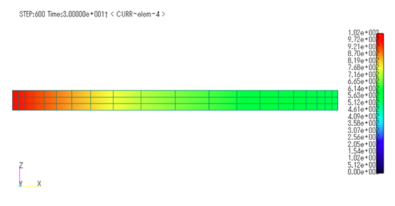
(b) Steady state

Fig.4 Current distribution in a conductor cross-section
(DC analysis using SUFCUR)

Since the objective of this condition is to obtain the steady state, i.e., DC current is applied, it is useless to perform DC analysis in TRANSIENT using SUFCUR, since the numerical transient state must also be included in the analysis.

A restart analysis can be performed using SUFCUR with the results obtained with PHICOIL as initial values. Let us apply this condition and analyze for 20 steps (0.1s). Fig. 5 shows the eddy current loss graph. As expected, the eddy current loss has a constant value of 0.01069W, which is consistent with the analysis using other methods. Of course, the current distribution in the conductor cross-section also agrees with PHICOIL.

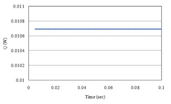
Fig.5 Eddy Current Loss Graph
(Restart DC analysis using SUFCUR with PHICOIL results as initial values)

Next, let us analyze the superposition of an AC current with a small disturbance on the DC current. The current is assumed to be a value of 0.1% of DC=3000A and AC=3A, 50Hz. First, let’s start from the beginning with SUFCUR. Since time increments are required to represent the AC waveform, it is necessary to perform many more steps than in the DC analysis described earlier, since the time increments are smaller. Here, the time increments are 20 divisions of a 50 Hz period = 1 ms, and 10,000 steps (10 s) are calculated. Fig. 6 shows the eddy current loss graph together with the results of the DC analysis using SUFCUR. The superposition of the AC current, which is about 0.1% of the DC current, does not affect the time constant, and the numerical transient state due to the DC current continues until steady state. Since the DC analysis reaches steady state in about 25s, the DC+AC analysis requires tens of thousands of additional calculation steps to reach steady state.

(a) Overall

(b) Enlargement

Fig.6 Eddy current loss graph
(DC+AC analysis using SUFCUR)

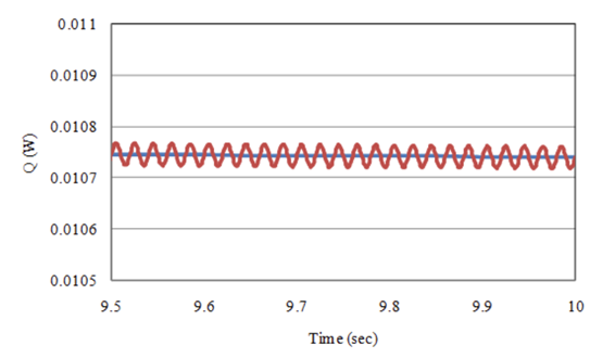
Since the model is a two-dimensional model, even 10,000 steps computation does not need much computation time, but with a three-dimensional model, tens of thousands of steps required just to exclude numerical transients is unrealistic. Therefore, let us perform a DC+AC restart analysis using SUFCUR with the results of the DC analysis using PHICOIL as the initial value. Although this is expected to be immediately steady, we will calculate 3 cycles at 50 Hz for confirmation. Fig. 7 shows the eddy current loss graph. Since the AC component is negligible, it has almost reached a steady state from the beginning of the calculation.

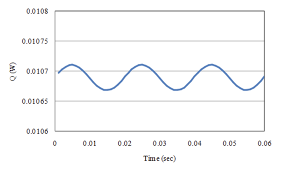
Fig.7 Eddy current loss graph
(Restart DC+AC analysis using SUFCUR with PHICOIL results as initial values)

The above are the methods of applying PHICOIL and SUFCUR for DC and DC+AC analysis of bulk conductors. The initial value used in the restart analysis should be close to the solution to be obtained in the restart analysis to quickly reach a steady state. In this case, the AC component was small, so the results of the DC analysis could be used as the initial value for the restart analysis. On the other hand, if a small DC component is superimposed on the AC component, it is considered that the time constant of the AC component is sufficient to reach a steady state, so it is recommended to perform DC+AC analysis from the beginning instead of restart analysis.