Summary

ELMCUR (element current source) is a current source that gives each element a current density or a current that passes through the element surface. It can be used when the surfaces and orientations of the elements are aligned. As an example, we will analyze the 3D static magnetic field verification model of the Institute of Electrical Engineers of Japan (Technical Report of the Institute of Electrical Engineers of Japan (Part II) No. 286, 3D static magnetic field numerical calculation technology, December 1988).

In this model, a magnetic field generated by a square coil is applied to an iron core of 100 mm $\times$ 100 mm $\times$ 200 mm (height), and the magnetic field distribution is calculated. The coil has a height of 100 mm, an inner width of 150 mm, and an outer width of 200 mm, and has R25 (inside) and R50 (outside) corners. It is assumed that the iron core has a relative permeability of 1,000 and a current of 3,000 AT flows through the coil. Considering its symmetry, the 1/8 region (x, y, z ≧ 0) is modelled.

Explanation

First, please define a two-dimensional mesh of the model as shown in Fig.1. For FEMAP input, use the FEMAP Property ID as the physical property number. Define Property ID in each area as shown in Fig.1. This mesh data is used as the input data to EMSolution as the file pre_geom2D.neu. Extension in the z direction is performed by file 2D_to_3D. Place the above two files and the execution control file input in the same directory, then execute EMSolution. On the EMSolution execution screen, select the execution menu to display the file dialog. Select the input.1 file and start execution. EMSolution creates a 3D mesh (Fig.2) based on pre_geom2D.neu and 2D_to_3D. The mesh data is output to the post_geom file. Of course, you can also enter the 3D mesh directly to start the calculation. In order to apply the source current with ELMCUR, the elements must be oriented in the same direction. In this case, we define the hexahedral element so that the current enters from surface 3 and exits from surface 5. In FEMAP, when defining each Surface, make sure that the first Edge is on the surface where the current flows.

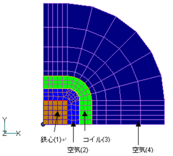
Fig.1　２D mesh

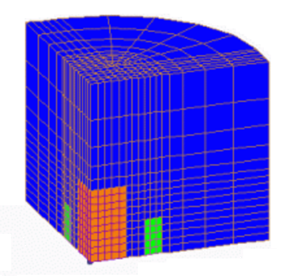
Fig.2 3D mesh

When you run the analysis, an output file output (included in the sample data as output.1) is created. In output, the summary of the input mesh, the calculation process, the calculation result, etc. are output. In addition, the echo of the input (input file) and the detailed convergence process of the ICCG method are output to the check file. If you see any anomalies during execution, check both files first. Also, an error message may be output to the stderr file. Various files are output to the execution directory, but if you plan to restart, leave the files as they are.

After execution, post processing is performed. If you use the input file included in the sample data, the output will be in Femap neutral format. If you are using FEMAP, first add the extension .neu to the file names post_geom, magnetic, and current. Next, since the post_geom does not contain property and material information, so please define it again on FEMAP. When you’re ready, load post_geom.neu with FEMAP first, then magnetic.neu and current.neu and display them.

Fig.3 shows the magnetic flux density distribution diagram, and Fig.4 shows the current distribution diagram in the coil. The unit of magnetic flux density is T, and the unit of current density is $A / m^2$. The current density is almost constant in the coil.

Next, let’s output the electromagnetic force by restarting. In this case, you only have to go through the post processing process. When re-starting, the output file such as output will be overwritten, so change the file name if necessary. First, change a part of the input file (input.2) to calculate the nodal force distribution, and re-execute EMSolution in the same directory. The electromagnetic force output part of the output file is shown in List.1.

This is the total electromagnetic force in each direction acting on the iron core and coils of the model (1/8 model). The electromagnetic force distribution is output to the force file. Fig. 5 shows the nodal electromagnetic force (unit N) acting to the iron core. Electromagnetic force appears only on the surface of the component with a constant magnetic permeability. Similarly, calculate the Lorentz force for the coil (input.3). Looking at the electromagnetic force (List.1) for each material shown in the output file, the electromagnetic force acting on the coil calculated from the above nodal force and the one obtained here are almost the same. In this case, the electromagnetic force distribution is output to the force_J_B file. Fig.6 shows the Lorentz force distribution ($N / m^3$) of the coil part.

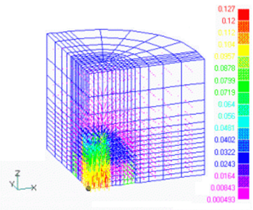
Fig.3 Magnetic flux density distribution（Ｔ）

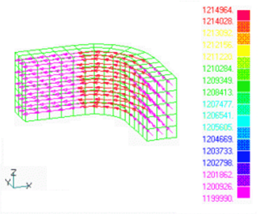
Fig.4 Current distribution in the coil ($A/m^2$)

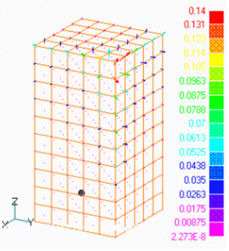
Fig.5 Nodal force distribution of the iron core (N)

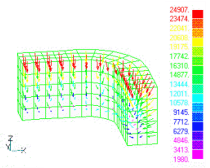
Fig.6 Lorentz force distribution of the coil ($N/m^3$)

List.1

• Coil electromagnetic force obtained from Lorentz force

*** Total J*B Forces ******************************************************************************* No. Fx(N) Fy(N) Fz(N) Mx(Nm) My(Nm) Mz(Nm) MAT 3 -2.68491e-01 -2.68527e-01 -2.22110e+00 -1.31787e-01 1.31785e-01 4.76718e-06 Total -2.68491e-01 -2.68527e-01 -2.22110e+00 -1.31787e-01 1.31785e-01 4.76718e-06

• Electromagnetic force obtained by nodal force

*** Total NODAL Forces and Torques ***************************************************************** No. Fx(N) Fy(N) Fz(N) Mx(Nm) My(Nm) Mz(Nm) MAT 1 1.55697e+00 1.57618e+00 1.06641e+00 -8.15032e-02 8.01692e-02 8.73281e-04 MAT 3 -2.83382e-01 -2.85275e-01 -2.15796e+00 -1.27305e-01 1.27377e-01 -7.65923e-05 Total 1.43569e+00 1.43574e+00 -1.06980e+00 -2.16243e-01 2.16245e-01 -5.32300e-06