Summary

In transient analysis, the number of steps to reach a steady-state solution is sometimes too large, even though the problem is known to converge to a steady-state solution in time, making it difficult to complete the analysis.　An example of such a case is given in ""Convergence of the solution to periodically applied magnetic fields". This problem converges to a constant steady-state solution. We showed that the convergence can be improved by changing the time step width. However, this required considerable ingenuity and did not lead to a fundamental solution. Here, we report a significant improvement by applying the SD-EEC (Singularity Decomposition-Explicit Error Correction) method to the Time-Periodic FEM (TP-FEM).

Explanation

1. Electrical circuit model

First, as a simple case, let us consider the case of an electric circuit only, which does not include the magnetic field calculation. EMSolution can also analyze only the circuit. When a voltage of 100 V at 1 kHz is applied to the voltage source, the time variation of the current is as shown in Fig. 2, and even if 1000 steps are calculated at 20 steps per period, it has not reached a steady state. This is due to the fact that the initial value was set to 0 in the analysis, but in general this is unavoidable. On the other hand, when the SD-EEC method is applied, as shown in Fig. 3, almost steady state is reached after half a period (10 steps), and you can see that the SD-EEC method is very effective. This analysis can be performed with AC steady-state analysis, and the result shows good agreement when compared with that result. However, when the circuit elements are nonlinear or when coupled with finite element analysis of a model that includes materials with nonlinearity such as iron, AC steady-state analysis is not applicable and transient analysis must be performed.

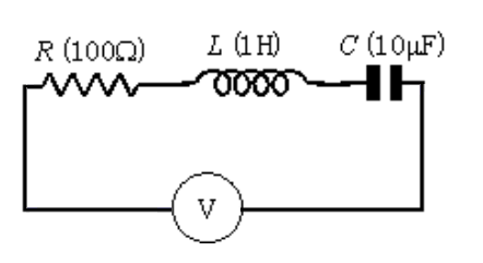
Fig.1 Electric circuit model

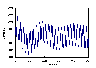
Fig.2 Time variation of circuit current

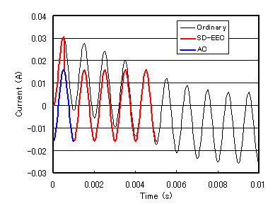
Fig.3 Convergence to steady-state solution when applying the SD-EEC method

Next, we apply it to the example of "Convergence of the solution to periodically applied magnetic fields".
In this problem, we analyze the Joule loss when a rotating magnetic field is applied to a circular Disk (Fig. 4). If the SD-EEC method is applied, convergence is reached in about 80 steps as shown in the red line in Fig. 5. Although a sharp peak appears every 15 steps, it is not physically meaningful because the correction is made every 15 steps by the SD-EEC method, and it appears in the calculation because the field changes discontinuously in time. Rather, it should be considered as a guide to the convergence of this method. This example can also be analyzed by steady-state eddy current field analysis, so there is no need to perform transient analysis, but it is necessary if the coil current oscillates or the circular disk is not uniform in the direction of motion.

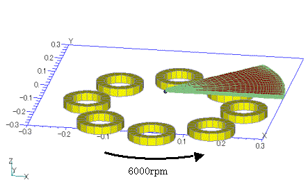
Fig.4 Circular Disk Model

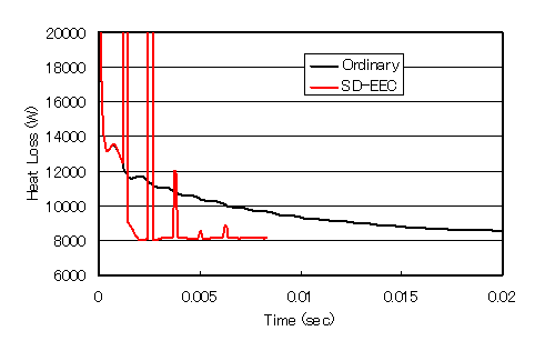
Fig.5 Joule loss in a circular Disk

2. Model with magnetic material and coil

This method can be applied to cases that include nonlinear magnetic characteristics and coupled circuits. An example model is shown in Fig. 6. A magnetic field is applied to a cube-shaped magnetic material by an external voltage source. The applied voltage is 1000(V){1-cos(wt)} including DC, and the frequency is 100 Hz. The analytical results of the coil current in this case are shown in Fig. 7. The normal method (No correction) is still far from steady state even after 100 steps, but the SD-EEC method (Correction) converges to steady state after 40 steps, which is after two corrections.

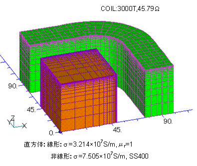
Fig.6 Magnetic cube model

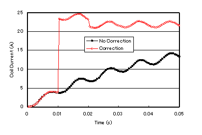
Fig.7 Coil current time variation

Next, a 10 µF capacitor is connected in series to the electric circuit to intentionally increase the time constant of the circuit. Figs. 8 and 9 show a comparison between the case with no correction (No correction), the case with correction of the last step of one cycle (End correction), and the case with correction of the step before half a cycle (Center correction). Note that in the Center correction, the second half of the cycle is not plotted, so almost twice as many steps are actually calculated.

No correction, of course, does not converge to the steady state easily, but even after 100 steps and 5 corrections in the End correction, the correction has not yet converged to the steady state. On the other hand, the Center correction has almost reached the steady state after 3 corrections (60 steps of calculation). Thus, the use of N_BACK is more effective than the SD-EEC method, which performs correction at each cycle. As a note, if the magnetic nonlinearity is not so strong as in this analysis and the analysis time to steady-state is determined by the time constant of the circuit, N_BACK, which corrects at the step before the half period, seems to be more effective. On the other hand, if the magnetic nonlinearity is strong, correction at the step before the half period is not necessarily effective, and correction at other steps back or correction at each period may be more effective.

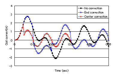
Fig.8 Coil current time variation when N_BACK is applied

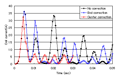
Fig.9 Joule heating time variation when N_BACK is applied

3. IPM motor model

This method can also be applied to motion analysis using the sliding method. It can be applied to synchronous motors, where the period of the power supply side and the period of the motion coincide. Let us apply this method to the IPM motor benchmark model used in "High-Speed, High-Accuracy Electromagnetic Field Analysis Techniques for Rotating Machines", IEEJ Technical Report No. 1094. Fig. 10 shows the applied model. The model is shown in Fig. 10. The model used is one with 6 poles and a capacity equivalent to 500 kW, driven at a speed of 1200 $min^{-1}$ and a frequency of 60 Hz. The motor consists of 11 permanent magnets of 40 $mm$ stacked in the axial direction for a total thickness of 440 $mm$. In the technical report, 120 degrees for two poles was modeled, but this time 60 degrees for one pole is modeled and the anti-periodic boundary condition is applied. In the axial direction, one half of one magnet is modeled, and the insulation between the magnets is treated as a 0.2 $mm$ air layer. The circumferential direction is divided into 60 segments of 1 mesh 1 degree. The calculation is performed by rotating the motor by 1 degree in 1 hour steps.

When performing load analysis on a normal PM motor, there is an internal induced voltage due to the permanent magnets, so it often takes time to converge to a steady state when performing a voltage source analysis. Therefore, in order to see the effect of the SD-EEC method, we will perform a voltage source analysis by applying a terminal voltage, whereas a current source analysis by applying an armature current was performed in the above technical report. The line voltage of 400 $V$ is given, the coil resistance is set to 0.01 $\Omega$ as appropriate since it was not specified in the above technical report, and the electrical phase angle (load angle) is set to 80 degrees, which is approximately 1 power factor. In the analysis procedure, the stator coil is first opened and a static magnetic field analysis of only the permanent magnet is performed, and then a voltage source transient analysis is performed using the results as the initial values. Fig. 11 shows the armature current, Fig. 12 shows the torque, and Fig. 13 shows the time variation of the Joule loss per magnet. The normal method (Normal) does not reach steady state even after 3,240deg (3 times the electric angle) calculations. In contrast, with the SD-EEC method (SD-EEC), corrections are made every 60 degrees of anti-periodic symmetry point, and steady state is reached after the third correction. As shown in the circular disk, the Joule loss shows sharp peaks at the first and second corrections but converges to a steady state after the correction.

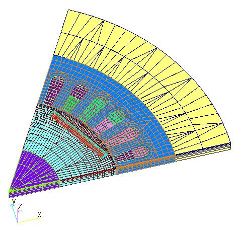
Fig.10 IPM Benchmark Model (60 degrees, 1/2 magnet model)

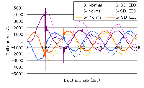
Fig.11 Electron current time variation

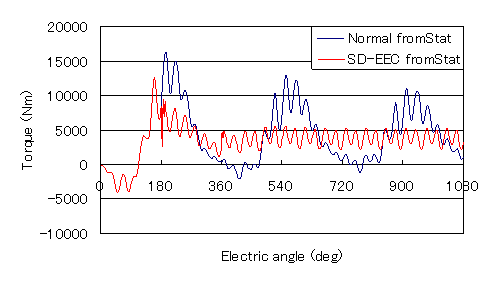
Fig.12 Torque time variation

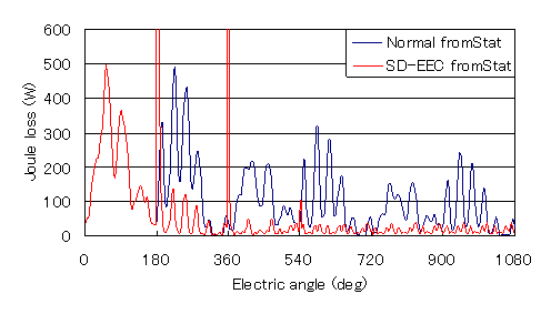
Fig.13 Time variation of loss per magnet

As described above, the SD-EEC time-periodic finite element method (TP-EEC method) is very effective for obtaining steady-state solutions. We hope you will make use of this method.

Currently, it cannot be applied to nonlinear or time-dependent circuit elements. It also cannot be used for analyses involving deformation motions. Until now, when the TP-EEC method was used with SUFCUR defined in the rotor (when one cycle correction was performed), the current values of SUFCUR diverged, but this can now be calculated by removing SUFCUR from the correction target.

How to use

The SD-EEC method is applied by simply entering N_CORRECT for the time step data in the input file to the conventional data. The method can be used only for transient (TRANSIENT) calculations. There are two types of periodicities: semi-periodicity, in which the sign is reversed at half cycle, and cyclicality, in which the DC component is included, and the value is the same at one cycle. In the case of semi-periodicity, enter the number of half-period steps with a negative sign. In the case of one cycle, enter the number of steps in one cycle. This can be applied to both CIRCUIT and NETWORK by inputting the circuit system. Although not related to the SD-EEC method, CYCLE can be used in the case where COIL moves and enter the number of steps in a magnetic field time period. In the case of the circular Disk example, this would be 15.

* NO_STEPS * INITIAL_TIME(s) * DELTA_TIME(s) * NO_DATA * CYCLIC *N_CORRECT * 101 0 0.0005 0 0 20

When using N_BACK, enter N_BACK after N_CORRECT ( N_BACK < N_CORRECT, half period before = 10 in the above example), and the SD_EEC method, which goes back N_BACK steps for correction, will apply.

* NO_STEPS * INITIAL_TIME(s) * DELTA_TIME(s) * NO_DATA * CYCLIC * N_CORRECT * N_BACK * 101 0 0.0005 0 0 20 10

When using this function, it is more stable to set THETA and THETA_NETWORK to the same 1, especially when using NETWORK, and also THETA_MOTION to the same 1 when using MOTION.

* ICCG_CONV * ACCEL_FACTOR * DIV_FACTOR * DIV_ITER * SOLVER * THETA * THETA_NETWORK * THETA_MOTION * 1e-006 0 100 100 0 1 1 1