Summary

This section describes an example of impact load analysis when a load greater than the steady-state torque is applied as an external torque at a certain time during steady-state operation.

Explanation

In "Dynamic Analysis of Brushless DC Servo Motor (ON-OFF Function by SWITCH Position)" the rotational motion of the rotor of a brushless DC servo motor is introduced as an example of coupled motion analysis using the Dynamic module, in which the analysis of the stable equilibrium point (the angle at which the torque crosses zero from positive to negative) and the analysis of the starting operation from that position are shown. In this way, EMSolution can analyze motors as close to actual phenomena as possible by coupling them with the equations of motion.

This section describes an example of impact load analysis when an external torque load greater than the steady-state torque is applied at a certain time during steady-state operation. In addition, since EMSolution ver. 10.2.3, a function to give the external torque as a time function has been added to the coupled equations of motion function, and this function is also used here. The Dynamic and Network modules of EMSolution are required to perform this analysis. In addition, we will perform the same impact load analysis using the coupled analysis with the feedback circuit described in "Coupled Analysis with Simulation Tool PSIM". This analysis requires the above modules and the PSIM Coupler module.

The analysis system is the same as that used in "Dynamic Analysis of Brushless DC Servo Motor (ON-OFF Function by SWITCH Position)" shown in Fig. 1 and is a two-dimensional nonlinear transient analysis. The boundary condition is set to a four counter-rotating periodic boundary condition. The calculation condition is not the ON-OFF input by SWICH, but the coil condition of "Application of COIL to motor windings" is slightly modified to use a 30Turn coil connected to a 3-phase AC voltage source of $30Vrms$ with a frequency of 100Hz as the voltage source, and the rotor speed is set to $3,000rpm$.

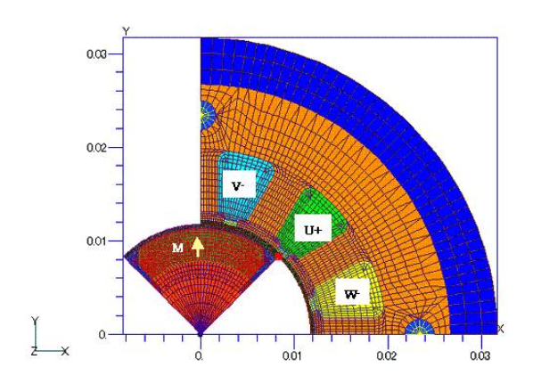
Fig. 1 Analysis model and mesh

To perform an impact load analysis, the steady state is first obtained by EMSolution.
For PM motors, the following calculation procedure is often used:

1. Static magnetic field analysis with magnetization given as input and zero armature current and terminal voltage
2. Transient analysis with the static magnetic field analysis of 1 as the initial value and armature current or terminal voltage applied as input

In the armature current input analysis, a steady state is reached relatively quickly, but in the terminal voltage input analysis, an internal induced voltage is induced by the magnetic flux of the rotor magnets, and it may take some time to reach a steady state. In both cases, the time-periodic finite element method (SD-EEC), described in "Fast Convergence to Steady-State Solution for Time-Periodic Problems", can be used to find steady-state conditions more quickly. In this motor model, the steady state is reached quickly even with a voltage source analysis.

Next, a coupled motion analysis is performed from this steady state to apply an impact load at a certain time. Restart analysis of the motion coupling is performed using the steady-state results as initial values. Restart analysis can also be performed from time 0. However, the terminal voltage phase must be matched and the angle of rotation of the rotor must be entered as the initial angle in the equations of motion. The first calculation is performed with the rated torque, and then an external load torque of 120% of the rated torque is applied at time 10 msec (when the machine angle rotates 90°) to see what kind of behavior will occur. In this case, the moment of inertia is assumed to be $2.e-4 kgm^2$. Note that the motion coupled analysis outputs the time, position (angle), velocity (angular velocity), and force (torque) in the motion file.

Fig. 2 shows the rotor rotation speed, Fig. 3 shows the rotor rotation angle, Fig. 4 shows the calculated torque waveform together with the external torque applied, and Fig. 5 shows the coil current waveform. Since this is an uncontrolled terminal voltage input analysis, when 120% of the steady-state torque is applied, the speed gradually drops from the steady-state speed of $18,000 deg/sec$, and the torque also decreases from the steady-state torque to a negative value, indicating that synchronization is lost.

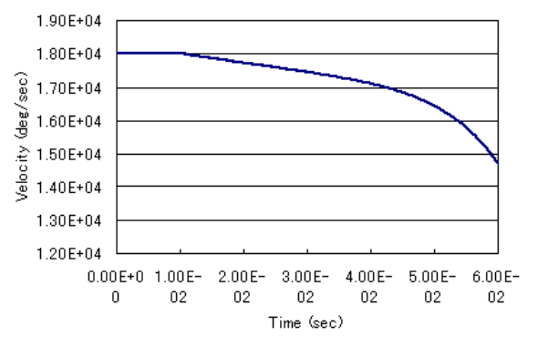
Fig.2 Rotor Rotation Speed

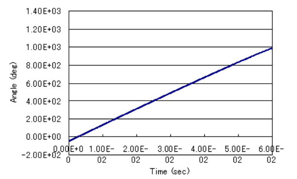
Fig.3 Rotor rotation angle

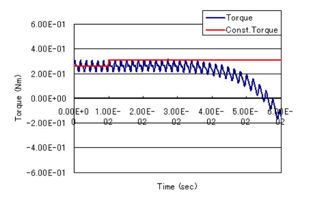
Fig.4 Torque waveform and external torque

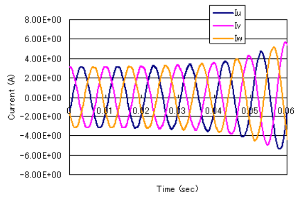
Fig.5 Coil current waveform

Next, the same analysis is performed using the PSIM Coupler module, which provides coupled analysis with PSIM. Fig. 6 shows a slightly modified version of the PSIM circuit used in section 3.2 of the "Simulation Tool: Coupled Analysis with PSIM".

The equivalent circuit for the equations of motion is shown in Fig. 7. The parameters of the equation of motion are set in the "Attribute" of the equivalent circuit of the equation of motion, which is a subcircuit. In this case, the equation of motion parameters in the EMSolution input file are ignored. The coupled analysis with PSIM can also be performed with the EMSolution steady-state solution as the initial value. In Fig. 7, the equation of motion is solved as an equivalent circuit in PSIM, but it is also possible to solve the equation of motion inside EMSolution and output the rotation speed and position to be passed to PSIM. The PSIM circuit diagram for this case is shown in Fig. 8. In both circuits, when converting the mechanical angle (deg/sec) to the electrical angle (rad/sec), 45 is first added to make the initial rotor position -45 degrees the electrical angle 0 degrees, and then doubled to convert the mechanical angle to the electrical angle, since the rotor has 4 poles. Furthermore, the initial phase angle of $Vu$ -120 degrees is added in the steady-state calculation of EMSolution, and unit conversion from deg/sec to rad/sec is performed and passed to the angle in the dqo-abc conversion block. In addition, $30Vrms$ is given as the amplitude of the steady-state voltage and the difference between the rotation speed and the speed command as the d-axis component as a $PI$ (proportional-integral) signal. For the external torque, the steady-state torque is first given as the load torque, and 120% of the steady-state torque is given at 10 msec. It seems that the variation in the initial stage of calculation is smaller if the motion is coupled in EMSolution.

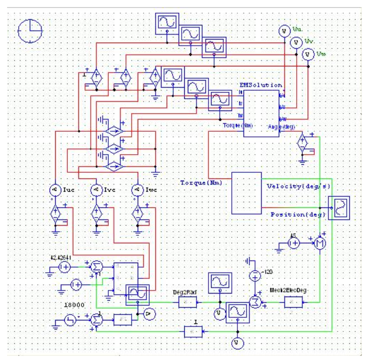
Fig.6 PSIM Circuit Diagram Subcircuit defines the equivalent circuit for the equations of motion

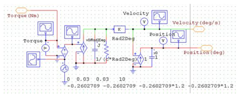
Fig.7 Equation of motion equivalent circuit diagram

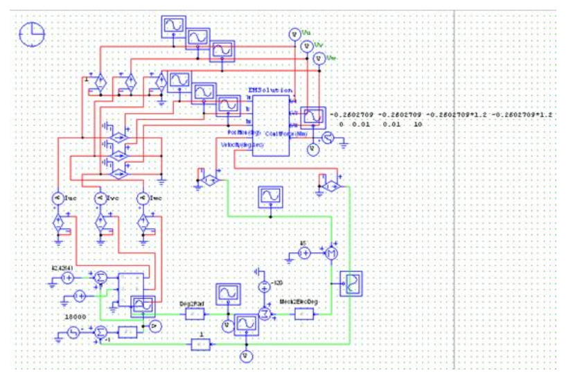
Fig.8 PSIM circuit diagram
In the case of motion coupling in the EMSolution

Fig. 9 shows the rotor rotation speed, Fig. 10 shows the rotor rotation angle, Fig. 11 shows the torque waveform together with the external torque, Fig. 12 shows the coil current waveform, and Fig. 13 shows the terminal voltage waveform. The speed fluctuates at the beginning compared to the Restart analysis with EMSolution alone, because the voltage values in PSIM are also slightly different. Even if 120% torque is applied, 10msec later at 20msec, it starts to oscillate around the specified value again, and the torque behaves in the same way. The terminal voltage also increases slightly at 10 ms, and the coil current increases accordingly, indicating that the control circuit is working properly.

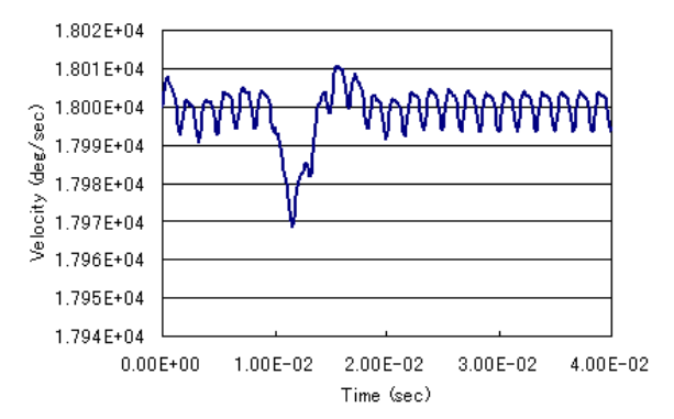
Fig.9 Rotor Rotation Speed

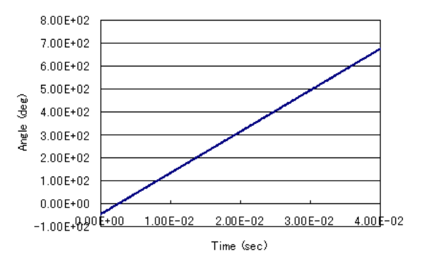
Fig.10 Rotor rotation angle

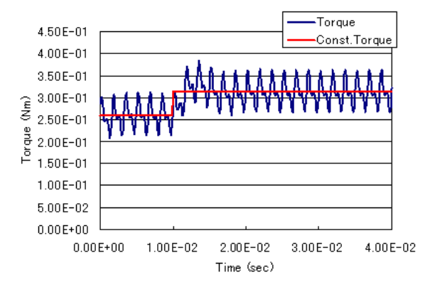
Fig.11 Torque waveform and external torque

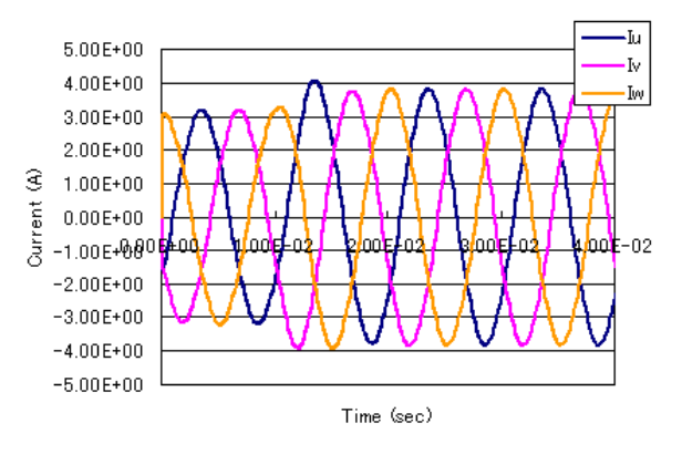
Fig.12 Coil current waveform

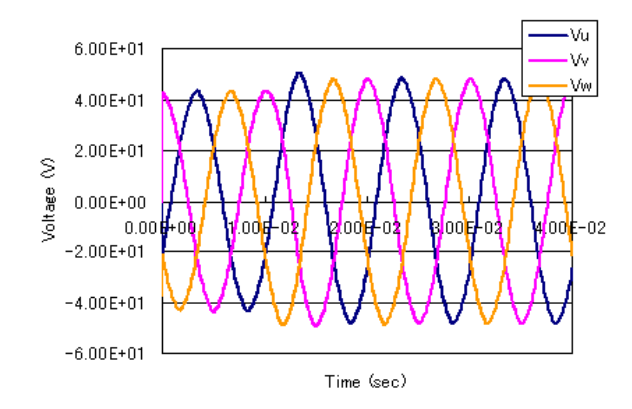
Fig.13 Pin voltage waveforms

Thus, we believe that we have shown that by applying an external torque over time and performing a motion coupled analysis, it is possible to perform an impact load analysis from a steady state. The motor used in this study, when analyzed with EMSolution alone, went out of synchronization, while the coupled analysis with PSIM showed that the motor returned to the specified speed by the control circuit. Although the model used in this study is a two-dimensional model and not very realistic, we hope you can understand some of the advantages of this method. We hope you will make use of this method.