Electromagnetic field analysis software

Electromagnetic field analysis software
Application of COIL to Motor Windings
- TOP >
- Analysis Examples by Functions (List) >
- Application of COIL to Motor Windings
Summary
In general, when analyzing motors, three-dimensional modeling is essential to accurately represent the winding geometry. However, the method of creating a three-dimensional mesh by piling up two-dimensional meshes is very time-consuming because the mesh must be divided according to the coil geometry. In addition, depending on the cross-sectional shape of the coil, it is necessary to use different magnetic field sources such as ELMCUR and SDEFCOIL. Therefore, we show here whether COIL can be applied as a motor winding.
Explanation
COIL can be defined independently of rotor and stator mesh division, making it easy to model windings. In the example treated here, a 90 degree 1/4 asymmetric two-dimensional model for cogging torque analysis of a permanent magnet motor is extended to three dimensions by stacking, and three-phase alternating current is given. For ease of viewing, the model is stacked as a two-dimensional model with 180-degree symmetry. The magnetic field sources applied to the coils are the ELMCUR magnetic field source (which is the reference case for comparison), the GCE block current element and the FGCE line current element of COIL. In addition, PHICOIL, which is usually used to apply current to bulk conductors, is also shown.
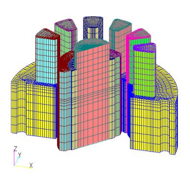
Fig. 1 shows the analytical mesh models used here: a model using ELMCUR(ELMCUR model), a model using GCE (also using ARC, hereafter referred to as the GCE model), and a model created using FGCE (also using FARC, hereafter referred to as the FGCE model). Note that the ELMCUR and PHICOIL models use the same mesh. The analytical mesh is 1/4 model, which is 1/2 in both angular and axial directions due to the symmetry of the model. In ELMCUR and PHICOIL models, the coil must be created with a finite element mesh, so the coil ends are ignored here. When created as in Fig. 1, the coil current flows in the Z-axis direction, and the coil is created from the bottom to the top of the Z-axis boundary. This is due to the fact that the boundary conditions on the top and bottom surfaces are set to Bn=0, and the current density continuity equation
$$\nabla \cdot J_o = 0$$
is satisfied. In this case, the coil current enters perpendicular to the top and bottom surfaces. On the other hand, when using COIL, GCE and ARC can only be created with a rectangular cross section, so it is not possible to accurately represent a coil shape with a trapezoidal cross section as defined in ELMCUR. Therefore, GCE and ARC are created so that GCE passes through the center of each coil for simplicity. In the FGCE model, the FGCE is given at each coil center.
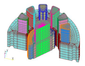
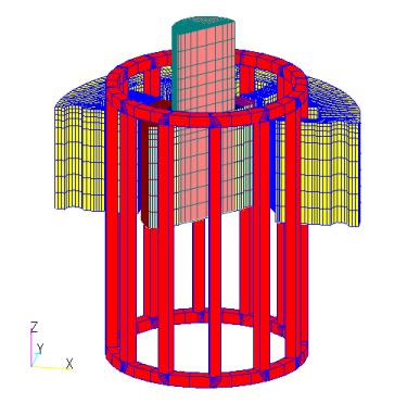
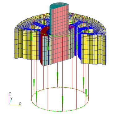
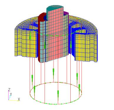
COIL requires all coils to be modeled because the symmetry of the finite element mesh does not apply to COIL. COIL, like ELMCUR and PHICOIL, must be defined to satisfy the continuity equation for current density, but since symmetry cannot be considered, all coils are connected as coil ends to form a closed loop. In the GCE model, ARC, the coil end, and GCE, the coil, are connected using ARC, and in the FGCE model, FARC, the coil end, and FGCE, the coil, are connected at right angles. Since the actual shape of the coil end is not known, it is virtually connected at 5.25 mm above the stator surface. The FGCE model was also created by extending the axial COIL to 5 m away from the stator surface to eliminate the effect of the coil end on the stator surface (hereafter referred to as the FGCE_far model). Note that even if COIL elements intersect or are defined on the same line, the current flow is not affected because the calculation is performed for each series. Fig. 2 shows the $U$, $V$, and $W$ coils defined in the GCE model.
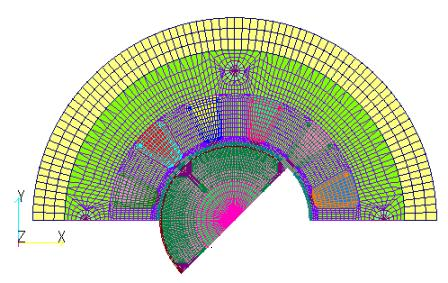
(a) XY plan view
(b) ELMCUR (PHICOIL) model
(c) GCE model
(d) FGCE model
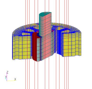
(e) FGCE_far model
(Axial extension up to 5 m)
Fig.1 Analysis mesh
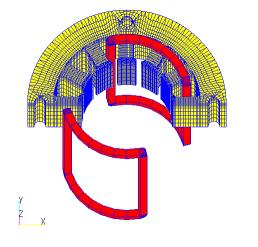
(i) U phase
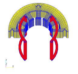
(ii) Phase V

(iii) W phase
Fig.2 $U$, $V$ and $W$ phases of a coil defined by the GCE model
The analysis conditions are as follows: a three-phase alternating current with a frequency of $100 Hz$ is applied to a 30-turn coil, each with an RMS value of $2 A$, and the rotor speed is set to $3,000 rpm$. The rotor and stator are assumed to be laminated iron cores, and eddy currents are not considered. The magnetization of the permanent magnet is set to 1.2T and the conductivity is given as $6.944 \times 10^5 S/m$ to calculate the eddy current loss of the magnet.
Fig. 3 shows the magnetic flux density distributions obtained for the ELMCUR, FGCE, and FGCE_far models, and Fig. 4 shows the eddy current vector distributions for those magnets. The same distribution is obtained for all magnetic field sources, and no differences are observed between the magnetic field sources. Since the magnets are calculated as bulk, large eddy current loops are created. The eddy currents do not change their position over time, but are large at the stator slot, forming a loop with that width. In general, the current is more inward in PHICOILs with bends or corners, but in this PHICOIL model, the end coils are ignored, so the current flows linearly and is not biased, resulting in a uniform current distribution across the coil cross section, similar to that of ELMCUR.
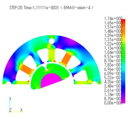
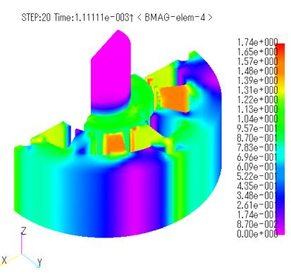
(a) ELMCUR model
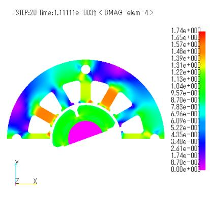
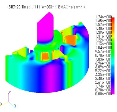
(b) FGCE model
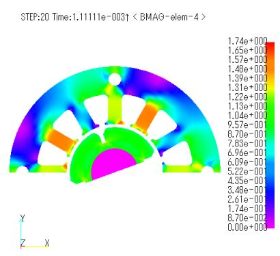
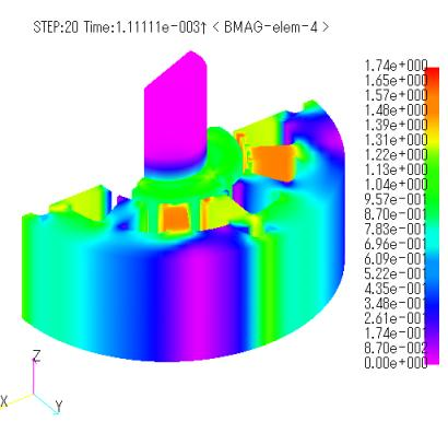
(c) FGCE_far model
Fig.3 Magnetic flux density distribution (20deg)
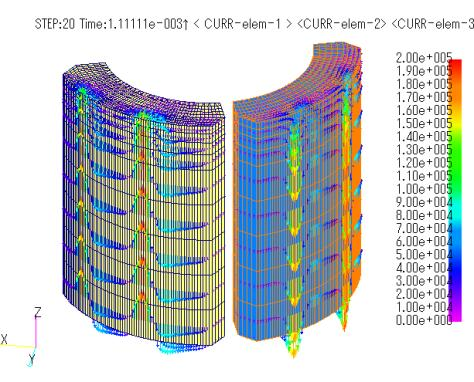
(a) ELMCUR model
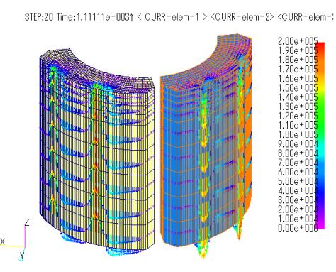
(b) FGCE model

(c) FGCE_far model
Fig.4 Eddy current vector distribution of magnet (20deg)
Figures 5 and 6 show the torque waveforms and the Joule heating waveform per magnet obtained for each model. Table 1 shows the average torque and eddy current loss per magnet obtained for each model. These show that the models are in good agreement regardless of the magnetic field source, although there are some differences. There is a small discrepancy between the ELMCUR and PHICOIL waveforms and the FGCE and GCE waveforms. This may be due to the fact that the FGCE and GCE models also take coil ends into account. The FGCE_far model, which eliminates the effect of coil ends on the stator surface, shows very good agreement with ELMCUR and PHICOIL. From this, it seems that if the coil ATs are matched, a very simple approximation with the FGCE line current is sufficient, even if it does not faithfully represent the coil geometry as ELMCUR does.

Fig.5 Torque waveform
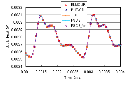
Fig.6 Joule heating waveform of one magnet
Table 1. Average torque vs. time-averaged heat generation of a single magnet
| Magnetic field source | Average torque ($Nm$) | Average heat generation per magnet per hour ($W$) |
|---|---|---|
| ELMCUR | 1.1589E-01 | 2.7740E-03 |
| PHICOIL | 1.1588E-01 | 2.7739E-03 |
| GCE | 1.1581E-01 | 2.7743E-03 |
| FGCE | 1.1550E-01 | 2.7732E-03 |
| FGCE_far | 1.1586E-01 | 2.7740E-03 |
The following is an example analysis using the ELMCUR, FGCE and FGCE_far models, using a model with overhangs on the magnets. The overhang is 10 mm above and below the stator. This means that the coil end is located at the overhang in the FGCE model, which takes the coil end into account. Fig. 7 shows the analytical meshes for the ELMCUR and FGCE models.
(a) ELMCUR model
(b) FGCE model
Fig.7 Analytical mesh with overhangs
Figures 8 and 9 show the magnetic flux density distribution and eddy current vector distribution of the magnet, respectively. The maximum magnetic flux density is 2.7T at the overhang corresponding to the slot in the stator. This is thought to be due to the effect of the overhang. At first glance, there seems to be no difference between the ELMCUR, FGCE, and FGCE_far models. However, while there is no difference in the joule heating waveform (Fig. 10), there is a slight difference in the torque waveform (Fig. 11). Table 2 shows the average torque and the average joule heating per magnet per time. Although the values are small, it can be said that the presence or absence of coil ends has an effect. Compared to the ELMCUR model without overhang, both torque and joule heating are considerably larger than the results without overhang.
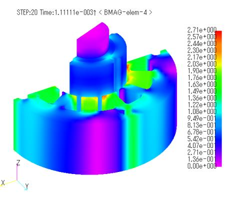
(a) ELMCUR model
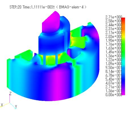
(b) FGCE model

(c) FGCE_far model
Fig.8 Magnetic flux density distribution with overhang (T)

(a) ELMCUR model
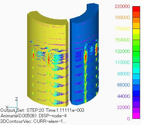
(b) FGCE model

(c) FGCE_far model
Fig.9 Eddy current vector distribution of magnet with overhang
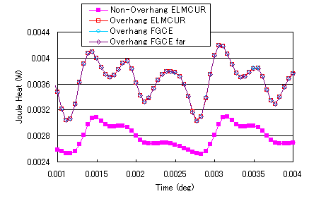
Fig.10 With overhang
Joule heating waveform of one magnet
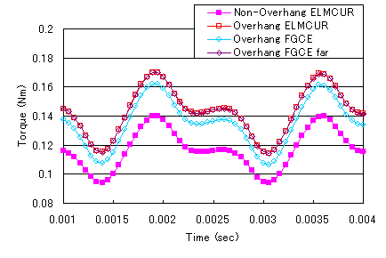
Fig.11 With overhang
Torque waveform
Table 2. Average torque with overhang and Comparison of time-averaged Joule heating of a single magnet
| Magnetic field source | Average torque ($Nm$) | Time soldier heat generation per magnet ($W$) |
|---|---|---|
| ELMCUR | 1.4219E-01 | 3.6578E-03 |
| FGCE | 1.3433E-01 | 3.6567E-03 |
| FGCE_far | 1.4191E-01 | 3.6574E-03 |
From the above, we believe we have shown that COIL is applicable as a motor winding, and that using FGCE, which is a line current approximation, is sufficient for torque and magnet eddy current loss calculations without using GCE, which is a rectangular form of COIL. However, care should be taken when the influence of coil ends becomes significant. Also, although the model used in this case had distributed windings, COIL can easily be used to model coil ends, even if they need to be modeled as in the case of concentrated windings. In addition, if coil ends are considered, eddy current losses generated in the stacking plane must also be considered because magnetic flux entering perpendicular to the stator surface is created, and iron loss is expected to increase. In this case, it is better to consider the eddy current loss generated in the in-plane direction of the laminated iron core using the homogenization method described in the iron loss calculation method, which is closer to the actual situation. We hope this will be helpful in your use of our products.
Download
No overhangs
・ input_ELMCUR.ems : Input file for ELMCUR model
・ input_PHICOIL.ems : Input file for PHICOIL model
・ input_GCE.ems : Input file for GCE model
・ input_FGCE.ems : Input file for FGCE model
・ input_FGCE_far.ems : Input file for FGCE_far model
・ pre_geom2D.neu : Stator mesh data
・ rotor_mesh2D.neu : Rotor mesh data
・ 2D_to_3D : 2D mesh stacking file
With overhangs
・ input_ELMCUR.ems : Input file for ELMCUR model
・ input_PHICOIL.ems : Input file for PHICOIL model
・ input_GCE.ems : Input file for GCE model
・ input_FGCE.ems : Input file for FGCE model
・ input_FGCE_far.ems : Input file for FGCE_far model
・ pre_geom2D.neu : Stator mesh data
・ rotor_mesh2D.neu : Rotor mesh data
・ 2D_to_3D : 2D mesh stacking file
Analysis Examples by Functions
Analysis of permanent magnet motors
- Application of COIL to Motor Windings
- Impact Load Analysis of Brushless DC Servo Motor
- Dynamic Analysis of DC Brushless Servo Motor (ON-OFF function based on SWICH position)
- Analysis of DC brushless servo motors (using switch function)
- Three-Dimensional Cogging Torque Analysis for Permanent Magnet Motors
- Two-Dimensional Cogging Torque Analysis for Permanent Magnet Motors
©2020 Science Solutions International Laboratory, Inc.
All Rights reserved.