Summary

In particular, in rotating machines with slot structures, magnetic flux density and the like are known to have both time and space harmonics. Briefly, time harmonics are observed when harmonics are superimposed on the fundamental wave input from the power supply, for example, when harmonics are superimposed on the current due to PWM voltage drive. Spatial harmonics are spatially distributed in a rotating machine and have a higher-order spatial distribution than the spatial distribution of the fundamental wave. For example, in a four-pole machine, the fundamental magnetic flux density is spatially distributed at 180 degrees for one period, and if third-order spatial harmonics exist, they are distributed for three periods compared to one period of the spatial distribution of the fundamental wave.

As a method for evaluating the electromagnetic excitation force of a rotating machine using frequency decomposition, the electromagnetic force can be calculated using the gap flux density for one electric angle period, and Fourier series expansion in space and time can be used to determine the electromagnetic force strength in spatial order and temporal order. This method is also used in sound and vibration analysis, and it is possible to check for resonance with the natural frequencies of structures such as stators.

In addition, consideration of the magnetic flux density distribution and eddy current distribution for each frequency-resolved order will provide clues to better geometry and other information. The results of frequency- resolved magnetic flux density distribution per order for IPM motors has already been published as Reference [1], but all functions of EMSolution do not support frequency decomposition function, and therefore we have not released them to the public. However, we have decided to release it with some limitations. The following functions are not yet supported.

• COIL_MOTION (not supported)
• Deformation region of mesh deformation DEFORM The deformation region also outputs order-specific results, but element deformation is not taken into account.

This function can be used as a post-processing function after the usual transient analysis has been performed: EMSolution internally decomposes the magnetic vector potential $A$ and the electric scalar potential $\phi$ into Fourier series and outputs the magnetic flux density and eddy current density for each order.

Explanation

The following is an example of frequency decomposition using an IPM motor. The magnetic flux density distribution by order for the IEEJ benchmark motor “D model (distributed winding)” and “D1 model (concentrated winding)” used in Reference (1) is shown. Figure 1 shows the analysis mesh. The two models are almost the same in size and dimensions, with (a) the D model with 4 poles and 24 slots and (b) the D1 model with 4 poles and 6 slots. The calculation conditions are 3Arms (rated) and $\beta$=25deg for the D model and 3Arms (near rated) and $\beta$=20deg for the D1 model.

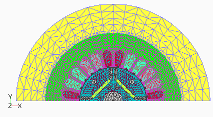
(a) D model (distributed winding)

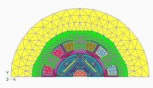
(b) D1 model (concentrated winding)

Figure 1 Analysis mesh

In general, the fundamental component makes the largest contribution to the average torque, and in a stator with an armature winding, the fundamental (1st order) is the largest in both time and spatial order. In a synchronous motor, the rotor is synchronized to the rotating magnetic flux by the fundamental wave, so the fundamental wave order in both time and spatial order is zero when viewed from the rotational coordinate of the rotor. The magnetic field to the stator is the sum of its own rotating magnetic field and the rotating magnetic field caused by the rotor, but to the rotor, there is no rotating magnetic field of its own, so only the rotating magnetic field caused by the stator appears. Therefore, the 5th and 7th orders of the stator correspond to the 6th order of the rotor, and the 11th and 13th orders of the stator correspond to the 12th order of the rotor. By frequency decomposition in this way, we can see the contribution of each order to the evaluation item.

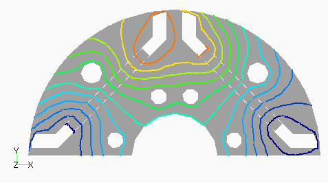
As flux distribution by order in the D model, Figure 2(a) shows the 1st order stator and (b) the 0th order rotor, Figure 3(a) shows the 3rd order stator and (b) the 12th order rotor. The stator 1st order and rotor 0th order represent the main flux flow, which can be seen even in a distribution that is not frequency-resolved. The stator 3rd order is for comparison with the D1 model, which is a concentrated winding. The 12th order of the rotor is due to the slot harmonics, and the spatial distribution on the rotor surface is also almost 12th order.

Note that the magnetic flux distribution is output in the static coordinate system for the stator and in the rotational coordinate system for the rotor, which is a coordinate system fixed to the rotor.

(a) Stator 1st order

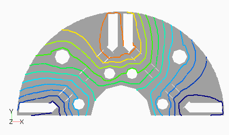
(b) Rotor 0th order

Figure 2 Magnetic flux distribution (D model)

(a) Stator 3rd order

(b) Rotor 12th order

Figure 3 Magnetic flux distribution 2　(D model)

Next, as magnetic flux distribution by order for the D1 model, Figure 4(a) shows the stator 1st order and (b) the rotor 0th order, Figure 5(a) shows the stator 3rd order and (b) the rotor 3rd order. The stator 1st order fundamental distribution does not appear to be as clean as the D model because of the odd number of slots. The 3rd order of stator matches the number of slots, so the 3rd order distribution can be seen spatially as well. The 3rd order rotor seems to have a 2nd order distribution instead of 3rd order, probably because the number of poles is 2nd order.

From these results, it can be seen that even in the same quadrupole machine, different orders appear in different distributions depending on the difference between distributed winding and concentrated winding.

(a) Stator 1st order

(b) Rotor 0th order

Figure 4 Magnetic flux distribution (D1 model)

(a) Stator 3rd order

(b) Rotor 3rd order

Figure 5 Magnetic flux distribution 2 (D1 model)

The frequency decomposition function in post-processing was introduced using examples.
We have shown the possibility of obtaining clues for changing the shape toward the target value by looking at the spatial distribution by order. We hope you will use this function.