Summary

Here is an example of analysis when multiple sliding surfaces are used. Although the analysis is a DC field eddy current analysis, it can be used equally well for magnetostatic, transient, and AC steady-state analyses. This model is a "linear motion conductor (Yamazaki model)" that is folded back to the lower side by removing the symmetry condition in the z=0 plane (Fig. 1). Of course, this is not necessary since the system is vertically symmetric, but it is done as a test calculation. In this case, two sliding planes are required (the analysis can be performed with one plane if the sliding surface is defined to enclose the motion conductor). The slide plane can be defined by two straight lines as shown in Fig. 1.

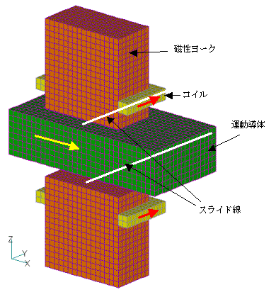
Fig.1 Linear motion conductor (Yamazaki model) model without upper and lower symmetry

Explanation

Input of sliding faces is shown in Table 1. SURFACE_MAT_ID=-1 to indicate multiple sliding face inputs; LINE_INPUT=-1 to specify that the sliding face is defined by a straight line. At this time, SLIDE_NDIV, FITNESS has no meaning because it is specified again on the bottom line. Then, after entering the number of sliding faces (NUMBER_SLIDING_FACES), enter each sliding face. For each sliding face, enter SLIDE_NDIV (number of divisions in the direction of motion), SURFACE_MAT_ID (ID number of the sliding face, a number that does not overlap with other MAT_IDs), FITNESS (If the distance between the mesh of the moving or rotating part and the split mesh of the sliding surface is smaller than the split width in the direction of sliding surface motion multiplied by this factor, both meshes are assumed to be perfectly coincident. Normally 0.5 is acceptable.　Normally 0.5 is acceptable.) and the positions of the two ends of the line, (SX,SY,SZ), (EX,EY,EZ) in meters. SLIDE_NDIV and FITNESS may be different for each face. At run time, the search is for edges in the mesh on which the straight line is defined. Therefore, the edges in the mesh must be on the straight line and they must be connected.

Table 1. Linear Designation of Multiple Sliding Faces (Linear Designation)

* CYCLIC * SYMMETRY * SLIDE_NDIV * SLIDE_MAT * FITNESS * LINE_INPUT * 1 1 32 -1 0.1 1 * DX(m) * DY(m) * DZ(m) * 0.08 0.0 0.0 * NUMBER_SLIDING_FACES * 2 * SLIDE_NDIV * SLIDE_MAT * FITNESS * 32 31 0.1 * SX(m) * SY(m) * SZ(m) * EX(m) * EY(m) * EZ(m) * 0.0 0.0 0.0125 0.0 0.06 0.0125 * SLIDE_NDIV * SLIDE_MAT * FITNESS * 32 32 0.1 * SX(m) * SY(m) * SZ(m) * EX(m) * EY(m) * EZ(m) * 0.0 0.0 -0.0125 0.0 0.06 -0.0125

Fig. 2 shows the eddy current density intensity distribution for a DC field eddy current analysis when the conductor is moving at $10 m/s$. Fig. 3 shows the magnetic flux density intensity distribution. The results are exactly the same as for the "linear motion conductor (Yamazaki model)", but the solution is symmetrical vertically.

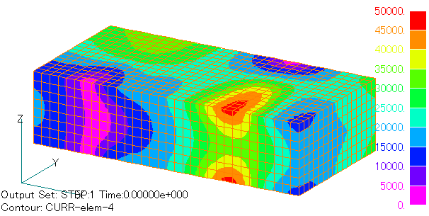
Fig.2 Current density intensity distribution in a moving conductor

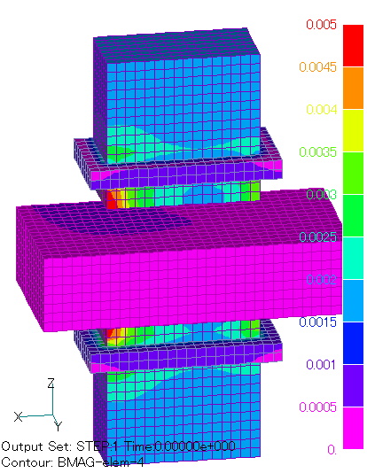
Fig.3 Magnetic flux density intensity distribution

As a second example, we will use a modified "Retarder model". As shown in Fig. 4, assume that there is another stator outside the rotor and the rotor rotates between the stator on both sides. In this case, sliding surfaces are specified on both sides of the rotor. This model is created by extending the 2D mesh shown in Fig. 5 in the z-direction. In this case, the sliding surfaces can be specified at the two points shown in the figure (mass elements in FEMAP). The point elements are converted to edge elements by 2D_to_3D file input. The MAT-IDs of these edge elements are 1 and 2. In this case, the input for the sliding surface is as shown in Table 2, where LINE_INPUT=0 and the MAT-ID of the edge element is specified in SURFACE_MAT_ID. Analysis results for a rotor at 100 rpm are shown in Figs. 6 and 7.

Table 2.　Linear designation (edge designation) for multiple sliding surfaces

* CYCLIC * SYMMETRY * SLIDE_NDIV * SLIDE_MAT * FITNESS * LINE_INPUT * 2 1 32 -1 0.1 0 * ANGLE(deg) * 30 * NUMBER_SLIDING_FACES * 2 * SLIDE_NDIV * SLIDE_MAT * FITNESS * 32 1 0.1 * SLIDE_NDIV * SLIDE_MAT * FITNESS * 32 2 0.1

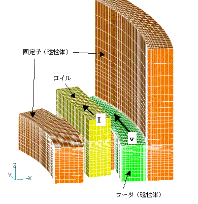
Fig.4 Retarder analysis model

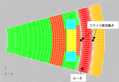
Fig.5 Two-dimensional mesh

Fig.6 Magnetic flux density distribution

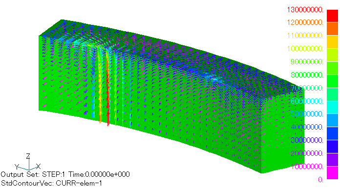
Fig.7 Current density distribution in the rotor