Summary

This model is a test problem for eddy currents in a moving conductor proposed by Mr. Yamazaki of Chiba Institute of Technology.

explanation

This model is a test problem for eddy currents in a moving conductor proposed by Mr. Yamazaki of Chiba Institute of Technology [Reference]　and shown in Fig. 1. A conductor (electrical conductivity $10^7 S/m$) moves at 10 $m/sec$ through a magnetic field source consisting of a coil wound around an iron yoke (specific permeability 1000). The model is symmetrical with respect to the z=0 and y=0 planes, and the 1/4 region is the finite element model domain. The boundary conditions are $B_n=0$ at z=0 and z=55, and $H_t=0$ at y=0 and y=60, as shown in Fig. 2. In the $x$ direction, the periodic anti-symmetry condition is assumed.

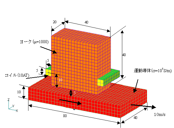
Fig.1 Analysis model

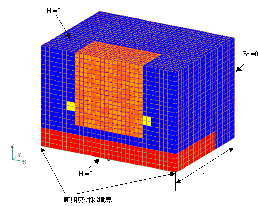
Fig.2 Analysis domain and boundary conditions

Fig. 3 shows the eddy current distribution obtained by the DC-filed eddy current field analysis. Fig. 4 shows a comparison with the transient analysis using the sliding method. In the transient analysis, there is almost no change between the second and fifth cycles. The transient analysis was performed using the backward difference method (q =1) to correspond to the DC-field eddy current field analysis, but it remains the same with q=2/3. Also, no fluctuations occur if the results of the DC-field eddy current analysis are used as the initial values in the transient analysis. In the DC-field eddy current analysis, the distribution is shifted about half a mesh in the direction of motion. This may be due to the fact that when obtaining the eddy currents post-processing, the transient analysis uses the time-centered difference, while the DC-field eddy current analysis uses the backward difference. We believe that the central difference is more accurate.

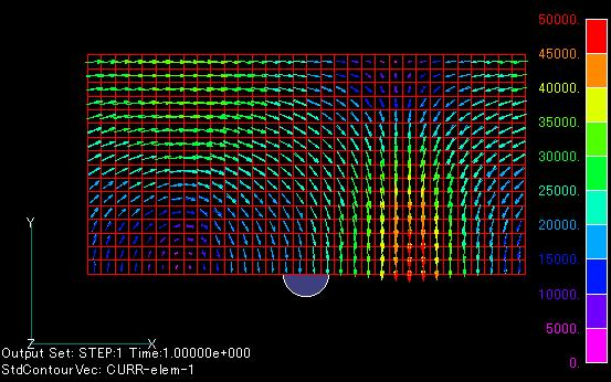
Fig.3 DC-field eddy current analysis
Eddy current distribution diagram
($A/m^2$)

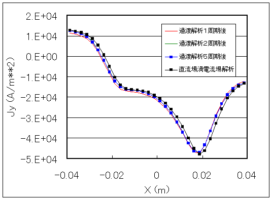
Fig.4 Eddy Current Distribution (y=1.25mm, z=8.75mm)

Fig. 5 shows the results of the DC-filed eddy current analysis, shifted by half a mesh in the upwind (opposite direction of motion) direction. In this case, the results of the transient analysis and the DC-filed eddy current analysis agree well. The results of the analysis with the mesh doubled in the direction of motion are also overlaid. Discrepancies can be seen near the current peaks, but elsewhere there is good agreement. This discrepancy is thought to be due to the improved accuracy resulting from the finer mesh. In the following example, the eddy current distribution is shown as it is in the backward difference. In DC-field eddy current field analysis, conductors are assumed to be uniform in the direction of motion, so there should be no problem if you understand that the distribution is off by half a mesh.

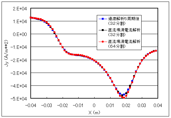
Fig.5 Eddy Current Distribution (y=1.25mm, z=8.75mm)
For DC-field eddy current analysis the abscissa is moved to the upwind side by half a mesh.

Next, Fig. 6 shows the magnetic field distribution. Fig. 7 shows the time variation of the electromagnetic force acting on the conductor in the direction of motion (which is the braking force) in the transient analysis and in the DC-field eddy current analysis. The transient steady-state value and the DC-field eddy current analysis result are in perfect agreement, both being 0.166033 $mN$. In addition, when the transient analysis becomes steady, the electromagnetic force is expressed in terms of (Joule loss/velocity), which is also in very good agreement at 0.166011 $mN$.

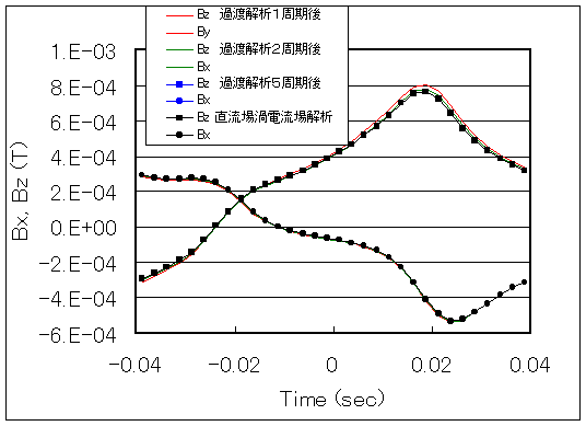
Fig.6 Magnetic field distribution
(y=1.25mm, z=8.75mm)

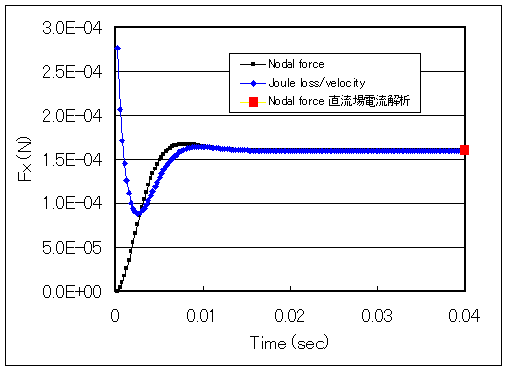
Fig.7 Total force acting on the conductor

As shown above, the results of the transient analysis and the DC-field eddy current analysis are almost identical, indicating the validity of this DC-field eddy current analysis. In this example, the calculation converges in about 2 cycles, so it can be performed in a transient analysis, but even so, more than 60 steps of analysis are required, and the DC field eddy current analysis, which requires a steady state in a single step, is highly significant.

Fig. 8 shows the change in magnetic flux density intensity when a transient analysis is performed at the same speed with the DC-field eddy current analysis as the initial value. The conductor is in motion, but the magnetic field at the same position in the stationary coordinate system is unchanged. This shows the validity of the DC-field eddy current analysis results.

Fig.8 Change in magnetic flux density intensity when a transient analysis is performed at the same movement speed with the DC eddy current analysis results as the initial value.

References

K. Yamazaki, “Generalization of 3D Eddy Current Analysis for Moving Conductors Due to Coordinate Systems and Gauge Conditions”, IEEE Transaction on Magnetics , Vol. 33, No. 2, March 1997.