Summary

At high frequencies or with high conductivity or permeability, the eddy current skin thickness may be very much smaller than the size of the object to be analyzed. In this case, if the properties are linear, the surface impedance method can be used. This eliminates the need for mesh division within the skin thickness and improves calculation speed and accuracy.

Explanation

In the "AC analysis including eddy currents", the conductor is assumed to have conductivity $\sigma=5.0×10^7 S/m$ and specific permeability 1. Assuming a frequency of 50 Hz, the thickness of the skin, d, is 10 mm from the following formula.

$$d=\sqrt{\frac{2}{\mu \sigma \omega}}$$

Assuming the same conductor dimensions (100 mm) of "AC analysis including eddy currents", this skin thickness is 1/10 of the coil dimension. Let us apply the surface impedance method to this.

When using the surface impedance method, define a surface on the surface of the conductor facing outward (toward the air region) as shown in Fig. 1. This is not required for symmetrical surfaces. Elements inside the conductor are excluded. Extension from two dimensions is done by 2D_to_3D. The mesh file pre_geom2D.neu defines line elements representing the copper surface. The physical properties of the surface elements are entered in the input file and execute the analysis.

In the surface impedance method, heat generation is output as a one-period average. Therefore, when outputting the total heat generation and its distribution, restart using input2 file of the sample data.

A portion of the output file output is shown in List.1. In this case, the output is the amount of heat generated by the surface impedance element. The voltages and heat generation are in fairly good agreement with the usual ones without surface impedance.

Fig. 1 and Fig. 2 show the eddy current distribution at the impedance surface. This distribution shows the surface current distribution that is the current integrated in the direction of the skin thickness (surface_current file). Fig. 3 shows the average surface heat generation density distribution (surface_heat file). Comparing the case without and with the surface impedance method, we can see that the distribution near the corners is very different. In general, the surface impedance method is less accurate near corners.

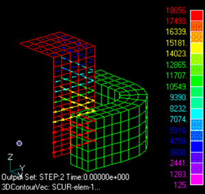
Fig.1　Current density distribution on impedance surface at 0 degree

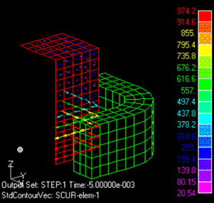
Fig.2　Current density distribution on impedance surface at -90 degree

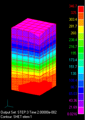
Fig.3　Surface heat generation density distribution$（W/m^2）$

List.1 File output

****************************************************************************** * Step No.1 Time -5.000e-003 sec * ****************************************************************************** *** Sources ********************************************************** ID No. Amplitude（Current） Voltage Flux 1 6.12303e-017 3.67318e+002 -8.26801e-002 *** Power Sources **************************************************** ID No. Current Voltage 1 6.12303e-017 3.67318e+002 ****************************************************************************** * Step No.2 Time 0.000e+000 sec * ****************************************************************************** *** Sources ********************************************************** ID No. Amplitude（Current） Voltage Flux 1 1.00000e+000 7.18802e+001 1.16921e+000 *** Power Sources **************************************************** ID No. Current Voltage 1 1.00000e+000 7.18802e+001 ****************************************************************************** * Total Joule heatin loss ( 1 cycle average ) in impedance_elements regions * ****************************************************************************** MAT No. Q （W） 101 1.6234e+000 ← Surface impedance Surface average Total heat generation Total 1.6234e+000