Electromagnetic field analysis software

Electromagnetic field analysis software
AC analysis using complex permeability
- TOP >
- Analysis Examples by Functions (List) >
- AC analysis using complex permeability
Summary
Ferrites are widely used as power inductors in small switching power supply circuits. In such applications, they are often used in the high-frequency range, and it is known that the loss increases as the frequency increases. Therefore, reducing the loss has become an issue. Generally, the magnetic properties of soft magnetic materials in the high-frequency range are expressed using the frequency characteristics of complex permeability. We have recently extended the AC steady-state analysis (AC analysis) to allow the setting of complex permeability.
Explanation
Complex permeability and loss
The basic equations of the so-called $j\omega$ method, a linear AC analysis without eddy currents using complex permeability, are expressed as follows:
$$\nabla×(\frac{1}{\dot{\mu}}×{\dot{A}})={\dot{J_0}} (1)$$
where A˙ is the magnetic vector potential, $\dot{J}$ is the input current density, $\dot{\mu}$ is the complex permeability, and dots ($\cdot$) denote complex numbers. The complex permeability is expressed as $\mu=\mu^{\prime} – j\mu^{\prime\prime}$, where $j$ is an imaginary number. The complex permeability has a frequency dependency, and in this AC steady-state analysis, $\mu^{\prime}$ and $\mu^{\prime\prime}$ are set at the frequencies to be analyzed. By using complex permeability, the magnetic flux density $B$ is phase delayed with respect to the magnetic field strength $H$. This phase delay causes a BH loop, and the area of which is the loss (core loss). The core loss $W(W/m^3)$ per unit time and unit volume is expressed by the following equation using $\mu^{\prime\prime}$.
$$W=\frac{\omega}{2\pi}\int HdB = \frac{1}{2}\omega\mu^{\prime\prime}H_0^2 (2)$$
where $\omega$ is the angular frequency and $H_0$ is the amplitude of the AC magnetic field $(H = H_0e^{j\omega t} )$. The actual core loss in the high-frequency range is generally said to consist of hysteresis loss, eddy current loss, and residual loss.
Analysis example
Referring to the reference [1], the analysis is performed using a toroidal coil with primary and secondary coils wound around a ring sample, as shown in Fig. 1. The material is a bulk sample of SUS430. The voltage is determined so that the average magnetic flux density in the sample is 5 mT, and AC voltages of 100 Hz, 1 kHz, and 10 kHz are applied. The calculation domain is 0.5 degrees in the angular direction and 1/2 in the vertical direction. The complex specific permeability is set with reference to the reference [1]. Up to 100 Hz and 1 kHz, $\mu^{\prime} > \mu^{\prime\prime}$, but at 10 kHz the $\mu^{\prime\prime}$ value exceeds the peak and conversely $\mu^{\prime} < \mu^{\prime\prime}$. For reference, we also show the results when a voltage with a frequency of 100 Hz is applied, giving a complex permeability with a value of only the real part.
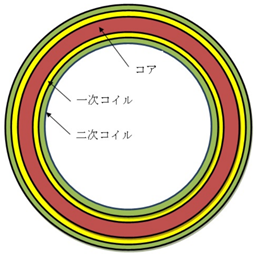
(a)Toroidal coil
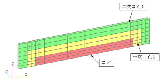
(b)Analysis area
(0.5 degrees in the angular direction and 1/2 in the vertical direction)
Fig.1 Verification model
Fig. 2 shows the current waveform. In order to compare the phase difference between the currents, a voltage waveform of the case with a voltage of 100 Hz and complex permeability having only the real part is also shown. Note that the amplitude of the voltage waveform increases by a factor of 10 as the frequency increases by a factor of 10, but the phase is the same. From this, when complex permeability is used, the current phase is slightly shifted at 100Hz, but is further shifted at 1kHz. It can be seen that at 10 kHz, where μ′′ < μ′′, there is a large shift. Fig. 3 shows the BH loop calculated from the current I and flux waveform $\Phi$. The BH loop is calculated from the following equations.
$$B = \frac{\Phi}{nS} (3)$$
$$H = \frac{nI}{l} (4)$$
where $n$ is the number of turns, $S$ is the sample cross-sectional area, and $l$ is the average magnetic path length. The effect of complex permeability at 100 Hz shows only a slight bulge in the current phase-difference curve, but at 1 kHz it is even larger, and at 10 kHz it is significantly larger. As explained earlier, the magnetic loss can be calculated from the area in the BH loop or from equation (2). Table 1 shows the magnetic loss calculated by the above method and inside EMSolution. Note that the $H_0$ used in equation (2) is the amplitude of H calculated in equation (4). It can be confirmed that they are in good agreement.
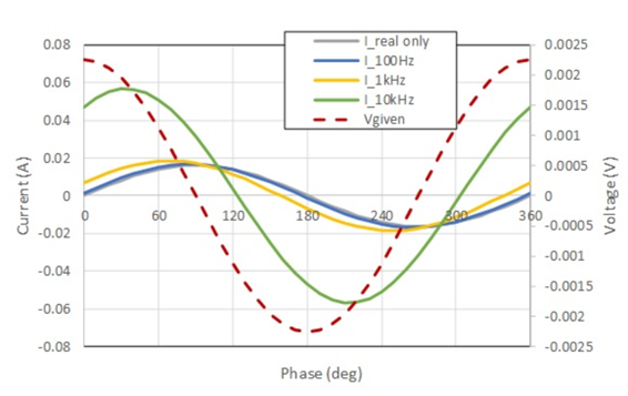
Fig. 2 Coil current waveform (A)
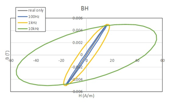
Fig. 3 Coil current waveform (A)
Table 1 Comparison of magnetic loss $(W/m^3)$
| frequency | BH loop area | (2) Equation | EMSolution |
|---|---|---|---|
| 100Hz | 1.908 | 1.892 | 1.918 |
| 1kHz | 104.04 | 103.68 | 104.57 |
| 10kHz | 7221.3 | 7171.2 | 7258.1 |
AC steady-state analysis using complex permeability is introduced briefly. This function is available for AC. As shown in reference [1], an analysis that considers both complex permeability and eddy currents is also possible. We hope you will make use of this function!
References
[1] : Liang, Hirata, Ota, Mitsutake, Kawase
Impedance Characteristics Analysis of Non-contact Magnetic Position Sensors, SA-07-72/RM-07-88 (2007)
How to use
To use complex permeability, set AC=2 in "2. Type of Analysis".
Set ANISOTROPY=1 in "16.1 Volume Element Properties" and Set the real part $\mu^{\prime}_r$ and the imaginary part $\mu^{\prime\prime}_r$ as the relative magnetic permeability in the next line.
For the calculation of magnetic loss, set AVERAGE=1 and IRON_LOSS=1 in "10.2 Output File" of EMSolution Hand Book, as in the case of time-averaged eddy current loss. In case of IRON_LOSS=1, the frequency must be set.
Download
・ input_complex_1kHz.ems
・ input_complex_10kHz.ems
・ input_complex_100Hz.ems
・ input_no_complex_100Hz.ems
・ inputPost_complex_1kHz.ems :Calculation of magnetic loss
・ inputPost_complex_10kHz.ems :Calculation of magnetic loss
・ inputPost_complex_100Hz.ems :Calculation of magnetic loss
・ pre_geom.neu :Mesh file
©2020 Science Solutions International Laboratory, Inc.
All Rights reserved.