Electromagnetic field analysis software

Electromagnetic field analysis software
About the multi-potential method
- TOP >
- Analysis Examples by Functions (List) >
- About the multi-potential method
Summary
In EMSolution, the analysis region is divided into a total potential region and a reduced potential region to facilitate the analysis by placing external magnetic field sources (called COIL in EMSolution) in the reduced potential region. This method is called the two-potential method. This section describes an extension of this method.
Explanation
magnetic field source need only be defined within the reduced potential region or outside the analysis domain, so its shape can be defined independently of the mesh. Therefore, the mesh can be easily created without being restricted by the shape of the current source. Also, because it is independent of the mesh, its position can be easily changed, and it can be used for current source motion analysis. In this analysis method, within the reduced potential, the magnetic vector potential is separated from the source potential due to the magnetic field source (COIL) and the reduced potential due to the magnetization of the magnetic body and conductor eddy currents in the total potential. The former is solved by integration of the Biot-Savart law and the latter by finite element method. The magnetic field near the coil is calculated independently of the mesh by integration of the Biot-Savart law, which is one of the advantages of this method, allowing for accuracy even when the mesh near the coil is coarse or the coil is located outside the mesh.
The multi-potential method, an extension of the two-potential method, uses different potentials in multiple reduced potential regions separated by a total potential region, as shown in Fig. 1. This allows the sliding method to place COIL in both stator and rotor sections using reduced potential regions. The multi-potential method is effective even when you do not use the sliding method. Since the integration of the Biot-Savart law in the reduced potential region can be limited to each region, it speeds up the calculation time. This is especially effective when complex COILs are defined.
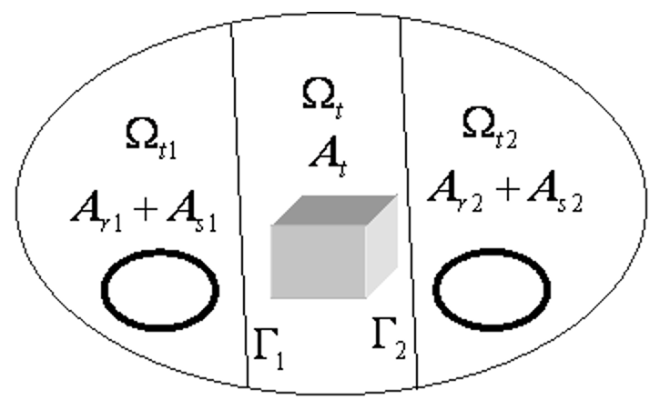
Fig. 1 Region partitioning for multi-potential method
As an example, suppose we perform an AC steady-state analysis with the model shown in Fig. 2, where the Cu Box represents the model domain (1/8 only), COIL 2 is inside the Cu Box, COIL1 and COIL3 are outside, COIL 1 and COIL3 are connected in series. Let us calculate the current induced in COIL 2 when an AC voltage is applied to COIL 1 and COIL 3.
Figures 3 and 4 show the results of the analysis of the eddy current density intensity distribution and spatial flux density intensity distribution on the Cu Box. Table I compares the conventional two-potential method with the multi-potential method in this example. The analytical results are in good agreement. On the other hand, the analysis time is reduced in Matrix Making and Post-processing, which may be due to the difference in the magnetic field integration at the boundary between the total and reduced potential regions in Matrix Making and the calculation of the spatial magnetic field in Post-processing. The amount of calculation increases in proportion to the number of COIL elements, so there is a large difference when complex COILs are defined.
Although not directly related to this method, the use of the THIN-ELEM option reduces the number of convergence times for the ICCG method from 823 to 401, and the calculation time is reduced to about 60%.
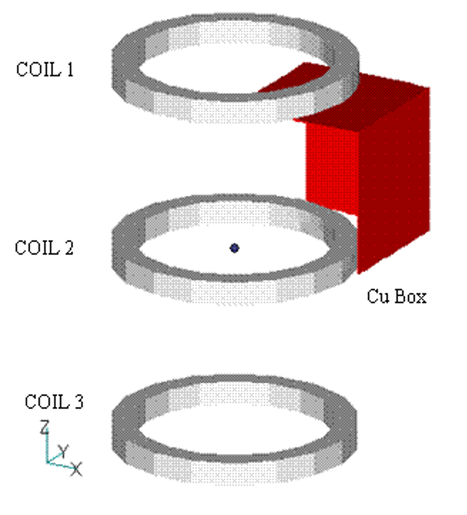
Fig.2 Analysis model
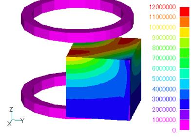
Fig.3 Eddy Current Density Intensity Distribution
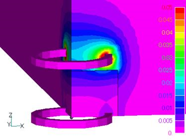
Fig.4 Magnetic flux density intensity distribution
Table I. Calculation Results and Computation Time
| 2-potential | Multi-potential | ||
| Coil current (A) | I I (real part) | 31.3413 | 31.3413 |
| I1 (imaginary part) | -21.6255 | -21.6262 | |
| I2 (real part) | -2.0858 | -2.0838 | |
| I2 (imaginary part) | 1.1980 | 1.1992 | |
| CPU Times ( s ) | Matrix Making | 16.4 | 14.0 |
| Post-processing | 20.9 | 16.8 |
This method is available in EMSolution r10.2.3 or later, including the case of the sliding method.
How to use
Setting volume element properties
Enter the reduced potential region number (1,2,…) in POTENNTIAL in "16.1.1. Properties of Volume Element". Each reduced potential region is assumed to be separated by a total potential region and not connected to each other. The total potential region is POTENTIAL=0.
Setting up an external current magnetic field source
In the COIL definition in "17.1. External Current Field Source", enter the reduced potential region number to which the COIL belongs. The default value is 1. Do not combine multiple COILs belonging to different reduced potential regions with CIRCUIT or NETWORK.
References
A. Kameari: “Regularization on Ill-Posed Source Terms in FEM Computation Using Two Magnetic Vector Potentials”, IEEE Transactions on Magnetics, Vol. 40, No. 2 ,2004, pp.1310-1313.
Download
・ input.ems
・ pre_geom.neu :Mesh file
Analysis Examples by Functions
External current magnetic field source
- About the multi-potential method
- Definition of COIL (external current field source) by hexahedral element mesh
- Magnetic field distribution calculation in a COIL-only model
- Circuit calculation with COIL (external current field source) only
- COIL inductance and electromagnetic force calculations
- Inductance Calculation for COIL (external current magnetic field source)
- Handling of inductance in external current field source (COIL)
- About COIL Move
- Problems with external magnetic field current sources in the case of translational periodicity
- Notes on the use of GCE (rectangular current element)
©2020 Science Solutions International Laboratory, Inc.
All Rights reserved.