Summary

This section introduces how to calculate the inductance and electromagnetic force of an external current magnetic field source (COIL).

Explanation

COIL is a mesh-independent feature that is easy to use. An example of an axisymmetric model is presented in "Inductance calculation for COIL (external current magnetic field source)", but here we will use a model that is 3-dimensional and includes magnetic materials as an example. The accuracy is verified by comparing the two-potential method (A-Ar method), in which the iron core portion is the total potential region and the coil and air portions are the reduced potential regions, with the case in which the entire region is solved with the total potential and the coil is defined with the surface-defined current source SDEFCOIL (A method).

Fig. 1 shows the excitation coil. The coil consists of four rectangular cross sectional straight sections (GCE) and arc sections (ARC). When determining the inductance and electromagnetic force, the integral regions in Fig. 1 are defined by the integral elements GCE- and ARC-. The analysis is performed in the 1/8 domain for symmetry. The integral element is defined as the part of COIL within the analysis domain. The magnetomotive force is set to 3000 AT and a linear static field analysis is performed.

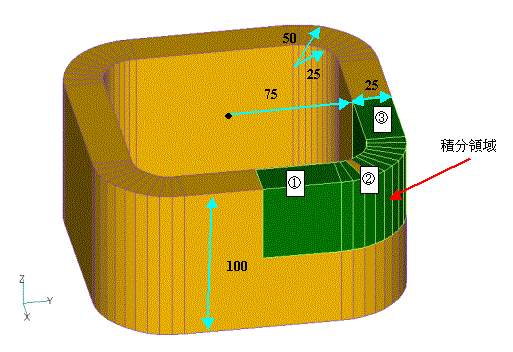
Fig.1　Excitation coil and integral domain

Fig. 2 shows the magnetic flux density intensity distribution obtained with the iron core (specific permeability 1000) and by using the A method. The result is almost the same as obtained using COIL. Table 1 shows the inductance calculation results using the A method. We analyzed the same problem with the boundary condition that Bn=0 and Ht=0 at far boundary. The results are almost the same, and the boundary condition is sufficient. Coil inductance is shown as a one turn equivalent value. The inductance can be calculated either by integrating A・J in the coil region and assuming it equals $LI$, or by taking the total magnetic energy (the total spatial integral of $B^2/2m_0$) as $LI^2/2$. Both methods are in good agreement. In EMSolution, the flux amount of $LI$ is output as the flux of the coil series. We also provide an option to calculate the magnetic energy (MAGNETIC_ENERGY option).

On the other hand, Table 2 shows the results obtained by the A-Ar method. The inductance is calculated and added internally, so the coil inductance includes the iron core effect. In this case, too, the analysis was performed with two types of boundary conditions, and the results are consistent. The results are also consistent with the results obtained by the A method. Without regularization, the ICCG method does not converge to $10^{-8}$, but the results are almost identical.

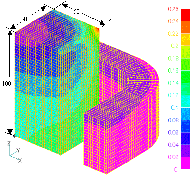
Fig.2　Iron core and magnetic flux density intensity distribution (the A method)

Table 1.　Inductance calculation results using the A method

Table 2.　Inductance calculation results by A-Ar method

Table 3 and 4 show the results of electromagnetic force calculations for both methods, showing the total force in each direction for each section ①, ②, and ③ in Fig. 1. It can be seen that the results of both methods are almost identical.

Table 3.　Electromagnetic force calculated by the A method

Table 4.　Electromagnetic force calculated by the A-Ar method

As shown above, the results of the A method with SDEFCOIL and the A-Ar method with COIL are almost in good agreement and both analyses are equivalent. In the above example, the mesh is sufficiently fine and the far boundary is sufficiently far away. However, please note that differences may appear if such conditions are not used.

How to use

To calculate the inductance of COIL internally in EMSolution, set the CALC_IND option to 1. The inductance calculation is performed by the MAKE_SYSTEM_MATRICES process.

* NODE_ORDER * EDGE_ORDER * METRIC_MAD * QUAD_TRI * CALC_IND * 1 1 0 0 1

To calculate the electromagnetic force of COIL, set COIL_FORCE in "10. Input/Output File" to 1. Please note that previously "11.1. Output Options" FORCE_J_B=2 was used, but this has been changed. The INTEG_OPT option was added as a new input data. With INTEG_OPT=1, the element integration point in a finite element is set to the element center point; with INTEG_OPT=0, the element Gaussian integration point is used. When INTEG_OPT =1 is used, computation time is significantly reduced. This option is also applicable for the calculation of conventional evaluation point magnetic fields. For calculations at a sufficient distance from magnetic materials or conductors, INTEG_OPT =1 is sufficient.

* MESH * CURRENT * MAGNETIC * FORCE_J_B * FORCE_NODAL * DISP * ELEM * HEAT * MAGNETIZATION * IRON_LOSS * E * COIL_FORCE * 1 0 0 0 0 0 0 0 0 0 0 1 * MESH * A * V * B * B_INTEG * J_Q * 0 0 0 0 0 0 * Q_AVERAGE * HEAT * MAG_FLUX * CUR_FLUX * 0 0 0 0 * FORCE_J_B * FORCE_NODAL * MAGNETIC_ENERGY * IRON_LOSS * 0 0 * XSIMMETRY * YSIMMETRY * ZSIMMETRY * ROTATION * 1 1 -1 1 * NO_POINTS * NO_MAT_IDS * NO_COIL_SERIES * INTEG_OPT * 0 1 1 1 * MAT_IDS * 15 * COIL_SERIES * 1

When calculating inductance with CALC_IND=1 or electromagnetic force with COIL_FORCE=1, the definition of integral elements is required. These definitions are done by LOOP-, GCE-, and ARC-. These have the same input format as LOOP, GCE, and ARC, respectively. However, the number of divisions and the number of Gaussian integral points must be entered at the end. These data are included in the coil definition. For example, the integral region in Fig. 1 is represented as follows. Since the upper half is defined here, CURRENT is also half. In this example, the number of coil turns is set to 100T.
NDIV (default value 1) is the number of divisions that divide the integral element equally in the current direction. Three-dimensional Gaussian integration is performed in the divided region. The electromagnetic force is output for each division; INT_X, INT_Y, and INT_Z are the number of integration points in each direction. The default values are 5, 5, and 3, respectively. INT_X and INT_Y are the number of integration points in the cross-sectional direction and INT_Z is the number of integration points in the current direction, with a maximum value of 12. The number of divisions and integration points required depends on the distribution of the magnetic field within the element, so increase the number of divisions and integration points as needed to make sure the results do not change. Since the electromagnetic forces are processed in POST_PROCESSING, you can change the number of integration points, etc., by performing post-processing in the restart calculation.

* GCE * CURRENT(A) * GCE 50 * XS(m) * YS(m) * ZS(m) * XE(m) * YE(m) * ZE(m) * 0.0875 0.0 0.025 0.0875 0.05 0.025 * W1X(m) * W1Y(m) * W1Z(m) * W2X(m) * W2Y(m) * W2Z(m) * 0.0 0.0 0.025 0.0125 0.0 0.0 * ARC * CURRENT(A) * ARC 50 * X(m) * Y(m) * Z(m) * RADIUS(m) * AXIAL_W(m) * RADIAL_W(m) * 0.05 0.05 0.025 0.0375 0.05 0.025 * ALPHA(deg) * BETA(deg) * PHI1(deg) * PHI2(deg) * 0.0 0.0 0.0 90 * GCE * CURRENT(A) * GCE 50 * W1X(m) * W1Y(m) * W1Z(m) * W2X(m) * W2Y(m) * W2Z(m) * 0.05 0.0875 0.025 0.00 0.0875 0.025 * W1X(m) * W1Y(m) * W1Z(m) * W2X(m) * W2Y(m) * W2Z(m) * 0.0 0.0 0.025 0.0 0.0125 0.0 * GCE * CURRENT(A) * GCE- 50 * XS(m) * YS(m) * ZS(m) * XE(m) * YE(m) * ZE(m) * 0.0875 0.0 0.025 0.0875 0.05 0.025 * W1X(m) * W1Y(m) * W1Z(m) * W2X(m) * W2Y(m) * W2Z(m) * 0.0 0.0 0.025 0.0125 0.0 0.0 * NDIV * INT_X * INT_Y * INT_Z * 1 5 5 3 * ARC * CURRENT(A) * ARC- 50 * X(m) * Y(m) * Z(m) * RADIUS(m) * AXIAL_W(m) * RADIAL_W(m) * 0.05 0.05 0.025 0.0375 0.05 0.025 * ALPHA(deg) * BETA(deg) * PHI1(deg) * PHI2(deg) * 0.0 0.0 0.0 90 * NDIV * INT_X * INT_Y * INT_Z * 1 5 5 3 * GCE * CURRENT(A) * GCE- 50 * W1X(m) * W1Y(m) * W1Z(m) * W2X(m) * W2Y(m) * W2Z(m) * 0.05 0.0875 0.025 0.00 0.0875 0.025 * W1X(m) * W1Y(m) * W1Z(m) * W2X(m) * W2Y(m) * W2Z(m) * 0.0 0.0 0.025 0.0 0.0125 0.0 * NDIV * INT_X * INT_Y * INT_Z * 1 5 5 3

As described above, when calculating the inductance and electromagnetic force of a COIL, the COIL information must be entered twice. On the one hand, the entire domain of the coil must be input as a conventional one, the coil that generates the magnetic field. On the other, the integral element does not create a magnetic field, but basically only the part within the finite element mesh region should be entered. For CIRCUIT or NETWORK, REGIONFACTOR is entered, and the inductance is integrated in the integral element, and using symmetry, REGION FACTOR is multiplied. The electromagnetic force is integrated only within the divided integral elements and output to the output file without REGION_FACTOR multiplication. The number of integrating elements is also included in the NO_ELEMENTS of the COIL data. This function can be applied to LOOP, GCE, and ARC, but not to line current elements such as FGCE and FARC.

Download

・ inputSDEFCOIL
・ inputCOIL
・ pre_geom2D.neu
・ 2D_to_3D

*This data cannot be run on the trial version due to the large number of nodes.