Summary

When calculating with an external current field source (COIL), the source field itself is not calculated in the reduced potential region. The magnetic energy of the source is not included in the reduced potential region, the inductance is calculated minus that amount. When analyzing magnetic fields and eddy currents with a constant current source, the inductance of the source has no effect on the analysis, so there is no problem with this. However, when the source is connected to a constant voltage source and the current itself is unknown, the electromagnetic field analysis is coupled with the circuit calculation and inductance is involved. For this reason, the air-core source inductance is assumed to be input as the external inductance. However, its handling is rather complicated, and we understand that some customers may have trouble with it. Here, we would like to explain its handling through an actual example.

Explanation

(1) Calculation of inductance by ELMCUR static magnetic field analysis

As a model for illustration, consider a two-dimensional axisymmetric model as shown in Fig. 1. Regions (1) and (2) are coil regions, and regions (3) and (4) are air regions (pre_geom2D.neu).
First, input ELMCUR into regions 1 and 2 and calculate the inductance of the coil. The coils are each 1000 turns, a current of 1A is applied to coil 1 and 0A to coil 2, and the self-inductance and mutual inductance of the coils are calculated from the interlinkage flux (input.1).

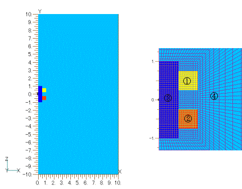
Fig.1 Test model

The coil definition is done as follows. The coil current is given in terms of current density, which is 4kA/$m^2$ for 1000 AT (the amount of current when 1 A is applied to the power supply, i.e., the number of turns).

* ELMCUR * SERIES_NO * NO_MAT_IDS * OPTION * 　ELMCUR 　　 1 　　　　 　 1　　　 　 1 * MAT_ID * IN_SURFACE * OUT_SURFACE * CURENT * SIGMA * 　 1 1 　　 　 2 4.00E+03 0.00E+00 * ELMCUR * SERIES_NO * NO_MAT_IDS * OPTION * 　ELMCUR 　　 2 　　　　 　 1　　　 　 1 * MAT_ID * IN_SURFACE * OUT_SURFACE * CURENT * SIGMA * 　 2 1 　　 　 2 4.00E+03 0.00E+00

The circuit system definition is as follows. The analysis area is for 1 degree, so REGION_FACTOR=360. This means that the circuit calculation is performed for the entire circumference. All external inductances and resistances are assumed to be zero. Power supply 1 is connected to coil 1 and power supply 2 to coil 2 to provide a constant current source. The current value is assumed constant at 1A for Power Supply 1 and 0A for Power Supply 2. TYPE=0 means a constant current source; TIME_ID=1 means to input its current change with ID number 1; TIME_ID=0 means current 0.

* CIRCUIT * CIRCUIT * NO_SERIES * NO_POWER_SUPPLIES * REGION_FACTOR * 2 2 360 * SERIES_IDS * 1 2 * SERIES_EXTERNAL_INDUCTANCE * 0 0 0 * SERIES_EXTERNAL_RESISTANCE * 0 0 0 * CONNECTION_MATRIX * 1 0 0 1 * PS_ID * TYPE * TIME_ID * INITIAL_CURRENT * 1 0 1 0 2 0 0 0 * END of CIRCUIT * END

When the calculation is run, the following flux quantities are output in output.1. The magnetic flux amount is 1000 turns (for 360 degrees in circumferential direction), and the value of ID No. 1 is the coil self-inductance, and the value of ID No. 2 is the mutual inductance.

*** Sources ********************************************************* ID No. Amplitude(Current) Voltage Flux 1 1.00000e+00 0.00000e+00 1.26862e+00 2 0.00000e+00 0.00000e+00 2.44741e-01

(2) AC analysis using ELMCUR

AC steady-state analysis is performed on the same model using ELMCUR (input.2). Region (3) is a magnetic material with a specific permeability of 1000, and a maximum value of 1A AC current is applied to coil 1. A constant voltage power supply is connected to the coil and its voltage is assumed to be zero. In other words, it is assumed to be in a short-circuit state. Assuming that the coil resistance is zero and the coil is a perfect conductor and the frequency is 100 Hz, the definition of the circuit system power supply is as follows. TYPE=1 represents a constant voltage power supply.

* PS_ID * TYPE * TIME_ID * INITIAL_CURRENT * 1 0 1 0 2 1 0 0

In the output.2 the following is shown: STEP1 represents phase -90 degrees and STEP2 represents phase 0 degrees, corresponding to the imaginary and real parts, respectively. Since we assume a perfect conductor state of the coil, the current flows only in phase 0. Since we assume a short-circuit state in coil 2, the current flows in the opposite direction so that the interlinkage flux is zero. It can be seen that a voltage of 1496V advanced by 90 degrees is required to flow 1A in coil 1. The impedance seen from coil 1 is $jwL=1.49649e+003j$, which is $1.49649e^{3}/(2p×100)=2.3817378$(H), different from that obtained in (1). This is due to the fact that region (3) is made magnetic material and coil 2 is short-circuited.Fig.2 shows the magnetic flux density distribution at phase 0. The magnetic flux is expressed in terms of the amount of magnetic flux for 1 degree.

********************************************************************** * Step No. 1 Time -2.5000000000e-03 sec * ********************************************************************** *** Sources ********************************************************* ID No. Amplitude(Current) Voltage Flux 1 6.12303e-17 1.49649e+03 1.45834e-16 2 -3.09262e-17 -5.81160e-09 -5.66348e-28 ********************************************************************** * Step No. 2 Time 0.0000000000e+00 sec * ********************************************************************** *** Sources ********************************************************* ID No. Amplitude(Current) Voltage Flux 1 1.00000e+00 0.00000e+00 2.38174e+00 2 -5.05080e-01 0.00000e+00 -9.24953e-12

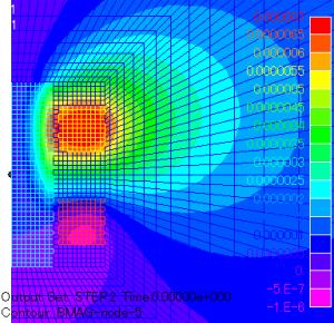
Fig.2 Magnetic flux distribution at phase zero

(3) AC analysis using external current field source COIL

The same condition as in (2) is calculated using COIL (input.3). First, change the material property definition as follows. That is, regions (1), (2), and (4) are set to reduced potential regions (POTENTIAL=1).

* NO_MAT_IDS * EXTEND_TOTAL * NO_SMAT_IDS * 4 0 0 * MAT_ID * POTENTIAL * B_H_CURVE_ID * SIGMA * MU * PACKING * 1 1 0 0 1.0 1 * MAT_ID * POTENTIAL * B_H_CURVE_ID * SIGMA * MU * PACKING * 2 1 0 0 1.0 1 * MAT_ID * POTENTIAL * B_H_CURVE_ID * SIGMA * MU * PACKING * 3 0 0 0 1.0 1 * MAT_ID * POTENTIAL * B_H_CURVE_ID * SIGMA * MU * PACKING * 4 1 0 0 1.0 1

The coil definition is as follows The LOOP (axisymmetric rectangular section coil) is used here to define it. Note that here the entire region is defined.

* SOURCE * SOURCE * COIL * SERIES_NO * TIME_ID * NO_ELEMENTS * MOTIN_ID * COIL 1 0 1 0 * LOOP * CURRENT(A) * RADIUS(m) * CENTER_Z(m) * RADIAL_W(m) * AXIAL_W(m) * LOOP 1000 0.75 0.5 0.5 0.5 * END of COIL * END * COIL * SERIES_NO * TIME_ID * NO_ELEMENTS * MOTIN_ID * COIL 2 0 1 0 * LOOP * CURRENT(A) * RADIUS(m) * CENTER_Z(m) * RADIAL_W(m) * AXIAL_W(m) * LOOP 1000 0.75 -0.5 0.5 0.5 * END of COIL * END

The circuit system is defined as follows Enter the self and mutual inductance of the air core obtained in (1) as the external inductance in the form of a symmetric matrix. No other changes are required.

* CIRCUIT * CIRCUIT * NO_SERIES * NO_POWER_SUPPLIES * REGION_FACTOR * 2 2 360 * SERIES_IDS * 1 2 * SERIES_EXTERNAL_INDUCTANCE * 1.26862e+000 2.44741e-001 1.26862e+000 * SERIES_EXTERNAL_RESISTANCE * 0.0 0.0 0.0 * CONNECTION_MATRIX * 1.0 0.0 0.0 1.0 * PS_ID * TYPE * TIME_ID * INITIAL_CURRENT * 1 0 1 0.0 2 1 0 0.0 * END of CIRCUIT * END

The results (output.3) are shown below, agreeing with the results of (2) by about 0.01%.

********************************************************************** * Step No. 1 Time -2.5000000000e-03 sec * *********************************************************************** *** Sources ******************************************************** ID No. Amplitude(Current) Voltage Flux 1 6.12303e-17 1.49701e+03 1.45885e-16 2 -3.09469e-17 -5.36612e-07 -5.22934e-26 *** Power Sources ************************************************** ID No. Current Voltage 1 6.12303e-17 1.49701e+03 2 -3.09469e-17 0.00000e+00 ********************************************************************** * Step No. 2 Time 0.0000000000e+00 sec * ********************************************************************** *** Sources ********************************************************* ID No. Amplitude(Current) Voltage Flux 1 1.00000e+00 0.00000e+00 2.38257e+00 2 -5.05418e-01 0.00000e+00 8.54045e-10 *** Power Sources ************************************************** ID No. Current Voltage 1 1.00000e+00 0.00000e+00 2 -5.05418e-01 0.00000e+00

(4) Analysis using NETWORK

EMSolution offers two methods of inputting circuit systems. One is the CIRCUIT format used so far, and the other is the NETWORK format described here. The CIRCUIT format requires input of the inductance, resistance, and CONNECTION matrix, which is not a problem for simple wiring such as in this example, but it lacks intuition. In contrast, the NETWORK format is easy to understand and can be entered just like connecting circuit elements. The NETWORK format also allows the input of capacitors and nonlinear circuit elements. The input in NETWORK format, equivalent to (3), is as follows (input.4): FEM represents elements in the finite element domain, which in this example correspond to coils (1) and (2). The external inductance is input by L and M. The constant-current power supply is defined by CPS and the constant-voltage power supply by VPS, and these are coupled at the circuit nodes.Fig.3 shows the block diagram.

* NETWORK * REGION_FACTOR * NETWORK 360 * FEM * ID * NODE1 * NODE2 * SERIED_ID * FEM 1 1 2 1 * L * ID * NODE1 * NODE2 * INDUCTANCE * L 2 2 3 1.26862e+000 * CPS * ID * NODE1 * NODE2 * TIME_ID * CPS 3 3 1 1 * FEM * ID * NODE1 * NODE2 * SERIED_ID * FEM 11 11 12 2 * L * ID * NODE1 * NODE2 * INDUCTANCE * L 12 12 13 1.26862e+000 * VPS * ID * NODE1 * NODE2 * TIME_ID * VPS 13 13 11 0 * M * ID * NODE1 * NODE2 * MUTUAL_INDUCTANCE * M 21 2 12 2.44741e-001 * END * END

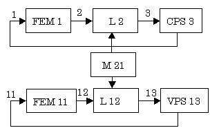
Fig.3 NETWORK wiring block diagram

The result of output.4 is exactly the same as 3 in terms of content, but the format is different. Current, voltage, and flux quantities are output for each circuit element, and flux quantities are output for the FEM and L elements only. Each quantity has a direction, which in this example is the direction of the arrow in Fig. 3. The voltage represents the generated voltage for each element, while the voltage drop and back EMF are represented by negative values. In a closed circuit, the total is zero. With COIL, the inductance is input as an external inductance, but the respective voltages and flux quantities are output separately. For example, in the current example, ID Nos. 1 and 2 correspond to coil (1), but in 3, the two values are output as the sum of the two. The value for the FEM element only is the induction from the total potential region, and the inductive component between the COILs is excluded.

********************************************************************** * Step No. 1 Time -2.5000000000e-03 sec * ********************************************************************** *** Network elements *********************************************** ID No. Current Voltage Flux 1 6.12303e-17 -7.77636e+02 7.57814e-17 2 6.12303e-17 -7.19377e+02 7.01040e-17 3 6.12303e-17 1.49701e+03 11 -3.09469e-17 -2.49092e+02 2.42743e-17 12 -3.09469e-17 2.49092e+02 -2.42743e-17 13 -3.09469e-17 0.00000e+00 ********************************************************************** * Step No. 2 Time 0.0000000000e+00 sec * ********************************************************************** *** Network elements *********************************************** ID No. Current Voltage Flux 1 1.00000e+00 0.00000e+00 1.23765e+00 2 1.00000e+00 0.00000e+00 1.14492e+00 3 1.00000e+00 0.00000e+00 11 -5.05418e-01 0.00000e+00 3.96442e-01 12 -5.05418e-01 0.00000e+00 -3.96442e-01 13 -5.05418e-01 0.00000e+00

Summary

In this section, we have presented a static magnetic field analysis using ELMCUR to obtain the inductance between coils and a calculation with COIL that uses this inductance as the external inductance. Although we discussed AC steady-state analysis, the method is the same for transient analysis; we performed equivalent calculations using ELMCUR and COIL and found that the results were in agreement. This demonstrates the validity of both methods. We also introduced two input methods, CIRCUIT and NETWORK, with NETWORK being the simpler of the two. In actual analysis, calculating inductance with ELMCUR or other methods is time-consuming and the advantage of COIL is considered to be small. Therefore, we plan to perform inductance calculation inside EMSolution in the future.

PS

The inductance of COIL can now be calculated inside EMSolution in r9.8.6 (8/29/2006). Please see " Inductance calculation for COIL (external current magnetic field source)"