Summary

EMSolution provides MAGNET as a finite element model of magnets. If the magnetization distribution of a magnet is not uniform, the magnet can be subdivided and a magnetization vector can be given for each property, or a magnetization vector can be given for each element. This section introduces the functions to set the magnetization distribution by inputting a sine function, which represents the magnetization distribution as a combination of sine waves, and by inputting a mathematical expression, which represents the magnetization distribution as a mathematical formula.

Explanation

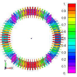
There are two types of magnetization orientations subject to sinusoidal function input: radial orientation (radial direction in cylindrical coordinate system) for a ring magnet shown in Fig. 1 (a) and parallel orientation (any direction in Cartesian coordinate system) shown in (b). Mathematical input can be applied to any magnet geometry.

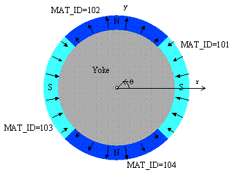
(a) Radial orientation

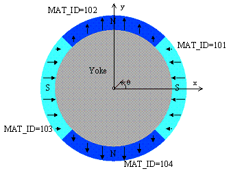
(b) Parallel orientation

Fig. 1 Ring magnet

The sine function input is described below. In the case of radial orientation in the cylindrical coordinate system shown in Fig. 1 (a), the radial ($r$-direction) component $M_r$ of magnetization is defined in the angular direction ($\theta$-direction). Suppose that the distribution is expressed as a Fourier series of sinusoidal functions as in equation (1). Generally, odd-order harmonics are used, where the magnetization distribution is symmetrical.

$$\displaystyle M_r ( \theta ) = M_{rs} \cdot \sum^{k_{max}}_{k=1,3,5,\cdot \cdot \cdot} b_k \sin \left( ( \frac{m}{2} ) k ( \theta – \theta_0) \right)　　　　　(1) $$

where $M_{rs}$ is the reference magnetization [$T$], $k$ is the harmonic order, $k_{max}$ is the maximum harmonic order, $b_k$ is the amplitude normalized by the reference magnetization of $k$-th order, and $m$ is the number of magnetic poles. Angle $\theta_0$ is the reference angle in the cylindrical coordinate system and corresponds to the position where the magnetization reverses (between poles). $\theta$ is the angle of the element center in the cylindrical coordinate system, and magnetization is assumed constant within the element. $m$ is the number of poles per 2$\pi$ and $\frac{m}{2}$ is the number of periods. The parallel orientation case shown in Fig. 1 (b) is expressed as in Eq. (2). The reference magnetization $M_s$ is a constant vector expressed in the local Cartesian coordinates of the respective physical property region. $\theta$ is the angle from the x-axis.

$$\displaystyle M(x,y,z) = M_s \cdot \sum^{k_{max}}_{k=1,3,5,\cdot \cdot \cdot} b_k \sin \left( ( \frac{m}{2} ) k ( \theta – \theta_0) \right)　　　　(2) $$

As Example 1, we show an analysis of the model in Fig. 1 with a magnetization distribution set up. The calculation conditions are: reference magnetization $M_s$ = 1.0 T, maximum harmonic order $k_{max}$ = 1 (fundamental component only), its amplitude $b_1$ = 1, and number of poles $m$ = 4. The specific permeability of the magnet is 1.02, the specific permeability of the yoke is 1000, and the outside is air. In the arrangement shown in Fig. 1, if the x-axis direction of the local coordinate is the x-axis direction of the overall Cartesian coordinate, the reference angle is $\theta_0$ = $\frac{\pi}{4}$.

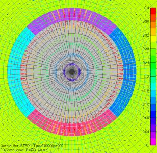
Fig. 2 shows the waveforms of the given magnetization $M_r$ and the analyzed magnetic flux density $B_r$ on the outer surface of the magnet. It can be seen that the magnetic flux density waveform on the outer surface of the magnet is nearly sinusoidal for radial orientation, while for parallel orientation, the magnetic flux density waveform is distorted between poles. The magnetization distribution (magnetization) and the magnetic flux density distribution (magnetic) are also shown in Fig. 3.

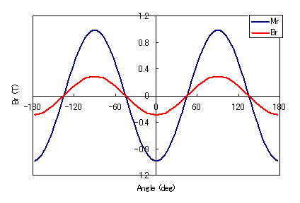
(i) Radial orientation

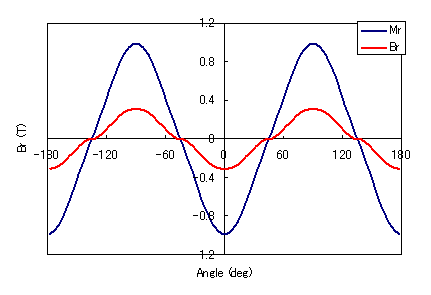
(ii) Parallel orientation

Fig. 2 Magnetization waveforms at the highest harmonic order
and magnetic flux density waveforms at the outer surface of the magnet

(i) Radial orientation

(ii) Parallel orientation

(a) Magnetization distribution (magnetization)

(i) Radial orientation

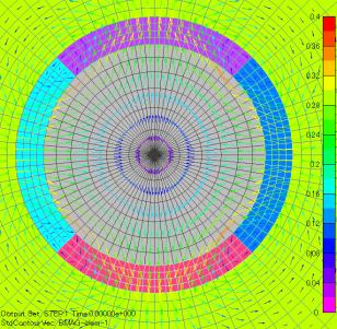
(ii) Parallel orientation

(b) Magnetic flux density distribution (magnetic)

Fig. 3 Magnetization and flux density distributions
for the highest harmonic order 1

Next, as Example 2, assume the radially oriented ring magnet model of Fig. 1(a) with $M_{rs}$=1.0T, $k_{max}$=5, $b_1$=1.0, $b_3$=0.25, and $b_5$=0.05. Fig. 4 shows the magnetization waveform and the flux density waveform on the outer surface of the magnet obtained by the analysis. The magnetic field distribution changes according to the magnetization distribution including harmonic components.

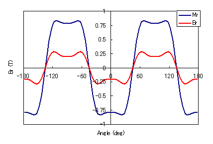
Fig. 4 Magnetization waveform of the 5th harmonic order
and magnetic flux density waveform
at the outer surface of the magnet (radial orientation)