Electromagnetic field analysis software

Electromagnetic field analysis software
Iron loss calculation by post-processing
- TOP >
- Analysis Examples by Functions (List) >
- Iron loss calculation by post-processing
Summary
Various methods have been devised to calculate the iron loss generated in laminated iron cores, which is the main component of loss in electrical equipment, using electromagnetic analysis. One simple method is to calculate the iron loss by post-processing from the magnetic flux density obtained by calculation. EMSolution has a function to calculate the iron loss approximately by post-processing.
Explanation
The iron loss calculation formulas here use either the maximum absolute value of the magnetic flux density or the method obtained directly from the magnetic flux density waveform. [Ref. 1]. In the following equation, the Cartesian coordinate system (x,y,z) is used, but a rotating magnetic field can also be considered if the cylindrical coordinate system (r,θ,z) is used. The iron loss $W_i$ is separated into eddy current loss $W_e$ and hysteresis loss $W_h$, as shown in Equation (1). Furthermore, eddy current loss $W_e$ is further divided into $W_{e\perp}$, returns in the thickness direction of the electromagnetic steel plate (lamination direction), and $W_{e\parallel}$, which flows through the steel plate surface (in the lamination in-plane direction).
$$W_i = W_e + W_h = W_{e\perp} + W_{e\parallel} + W_h \tag{1}$$Eddy current loss $W_{e\perp}$ and hysteresis loss $W_h$ in the stacking direction are calculated post-processing from the magnetic flux density history obtained by FEM analysis. The in-plane eddy current loss $W_{e\parallel}$ in the stacking plane is directly obtained using the eddy current $J_e$ obtained by FEM analysis.
Calculation method ① : Method obtained from the maximum value of magnetic flux density
When an alternating magnetic field of a single frequency $f$ and amplitude $B_{max}$ (the maximum value of magnetic flux density) is applied, the iron loss is calculated from the following iron loss estimation formula.
$$\displaystyle W_i = W_{e \parallel} + ( w_{e \perp} + w_{h} ) \Delta V_i = W_{e \parallel} + \left( K_e f^\alpha B_{max}^\beta + K_h f B_{max}^\gamma \right) \Delta V_i \tag{2}$$where $\Delta V_i$ is the volume ($m^3$) of finite element i, $K_e$ is the eddy current loss coefficient ($W/kg/T^2/Hz^2$), and $K_h$ is the hysteresis loss coefficient ($W/kg/T^2/Hz$). In addition, $\alpha$, $\beta$, and $\gamma$ are coefficients representing powers, and are set to $\alpha = \beta = \gamma = 2$ by default. Since the magnetic flux density waveform is assumed to be sinusoidal, the amplitude is calculated as the absolute value of the maximum value of the magnetic flux density. The eddy current loss $W_{e\parallel}$ in the lamination plane is calculated directly from the FEM analysis by the following equation.
$$\displaystyle W_{e \parallel} = \frac{1}{T} \int^T_0 \int_{iron} \frac{ | J_e |^2}{\Sigma_\parallel} dv dt \tag{3}$$ $$\Sigma_\parallel \equiv \alpha \sigma_s 、 \Sigma_\perp \equiv 0 \tag{4}$$where $T$ is the period $(s)$, $\alpha$ is the occupancy factor, and $\sigma_s$ is the conductivity of the iron section ($S/m$). This means that in FEM analysis, only eddy currents in the in-plane direction of the lamination are calculated considering the occupancy factor.
Calculation method ②: Direct method from magnetic flux density waveform
If the magnetic flux density waveform is not sinusoidal or contains minor loops, the approximation accuracy of equation (2) is not high. In this case, the eddy current loss $W_{e\perp}$ in the stacking direction is calculated by the following equation.
$$\displaystyle W_{e \perp} = \frac{K_e D}{2 \pi^2} \int_{iron}\frac{1}{N}\sum^N_{k=1} \Biggl[ \biggl(\frac{{B_x^{k+1} – B_x^k}}{\Delta t}\biggr)^2 + \biggl(\frac{{B_y^{k+1} – B_y^k}}{\Delta t}\biggr)^2 \Biggr] dv\tag{5}$$where $D$ is the density of the iron core ($kg/m^3$), $N$ is the number of iterations (number of samplings) per cycle, $\Delta t$ is the time increment ($s$), and $k$ in the superscript of $B$ represents the time step. The eddy current loss expressed in equation (5) excludes the term related to the z component of the magnetic flux density in the stacking direction. This is because it represents the eddy current loss flowing in the stacking plane induced by the magnetic field in the stacking direction, which can be obtained from the FEM analysis using equation (3). The hysteresis loss $W_h$ is calculated by the following equation.
$$\displaystyle W_h = \frac{K_h D}{T} \sum_{i=1}^{N_E} \frac{\Delta V^i}{2} \Biggl( \sum_{j=1}^{N_{px}^i} ( B_{mx}^{ij} )^2 + \sum_{j=1}^{N_{py}^i} ( B_{my}^{ij} )^2 + \sum_{j=1}^{N_{pz}^i} ( B_{mz}^{ij} )^2 \Biggr)\tag{6}$$where $N_E$ is the number of elements in the iron core region, $N_{px}^i$, $N_{py}^i$, and $N_{pz}^i$ are the number of maxima and minima for the time variation of each component of the magnetic flux density in the i-th finite element, and $B_{mx}^{ij}$, $B_{my}^{ij}$, and $B_{mz}^{ij}$ are the amplitudes of the major and minor loops, which are determined from all maxima and minima of the magnetic flux density waveform in the manner shown in Fig. 1. In doing so, the square of the amplitude of the magnetic flux density in a given loop is added twice and divided by two after the addition. This means that the hysteresis loss for major and minor loops is determined by the same algorithm.

Fig. 1 Method for determining major and minor loop amplitudes in Eq (6)
The iron loss coefficients $K_e$ and $K_h$ are obtained from the measured iron loss $W_i$ at each frequency $f$ and magnetic flux density $B$. A $f (Hz) – Wi/f (W/kg/Hz)$ graph at a representative magnetic flux density (e.g. $B_m$ = 1T) is created, the slope of which is a linear approximation of $K_e$ and the intercept is used as $K_h$. When analyzing a laminated iron core by applying the homogenization method (PACKING) and calculating iron loss, the magnetic flux density of the iron section of the laminated iron core described in “Analysis of Laminated Iron Core by Homogenization Method and Output of Magnetic Flux Density of Iron Section of Laminated Iron Core” is used.
Next, as a concrete example, we show the iron loss calculation of a DC brushless motor from “Analysis and Experiment of Model for Validation of Iron Loss Calculation Method”[Ref.1]. (Fig. 2). This model is used to measure the iron loss due to the rotor’s permanent magnet when the rotor is forced to rotate without coil windings in a laminated iron core consisting of 50A1300 non-oriented electromagnetic steel plates for both the stator and rotor, and to compare and verify the results with those obtained by analysis. For the iron loss calculation, we used the results calculated at a machine angle of 180 degrees, which is one cycle of $B_r$, to use the magnetic flux density component in cylindrical coordinates. The following are the results of two- and three-dimensional nonlinear static magnetic field analysis in which the laminated iron core is treated as an iron core with zero conductivity, and nonlinear transient analysis including eddy currents in which the laminated iron core is approximated by the homogenization method (PACKING). Here, the BH curves are in the L+C direction (averaged over the rolling direction and its perpendicular direction), and the stacking direction is in the z direction. However, the occupancy ratio was assumed to be 98.5% since it is not specified in the literature. The comparison is made at the motor rotational speed of 1500 rpm.
Fig. 3 shows the eddy current loss and hysteresis loss distribution in the stacking direction of the 3D static magnetic field analysis results obtained by post-processing. Fig. 4 shows a comparison of the calculated and experimental iron loss results, and Table Ⅰ shows the breakdown of the iron loss. Compared to the results of calculation methods ① and ②, the value of calculation method ① is smaller. This may be due to distortion of the magnetic flux density waveform and minor loops. Fig. 5 shows the distribution of eddy current loss in the in-plane direction, which is the result of a three-dimensional nonlinear transient analysis including eddy currents using the homogenization method. The eddy currents are concentrated at the upper edge, although the value is small.
Note that calculation method ① assumes an alternating magnetic field as the applied magnetic field. Therefore, even though the magnetic flux density of the rotor does not change with time with respect to position, the maximum absolute value of the magnetic flux density is used, resulting in the calculation of iron loss that is not actually generated. For this reason, the values for the stator section only are used for comparison. An example of analysis using a simple model in which an alternating magnetic field is applied to a laminated iron core is shown in “Analysis of Laminated Iron Core by Homogenization Method and Output of Magnetic Flux Density of Iron Section of Laminated Iron Core”. There, both calculation methods ① and ② show good agreement.
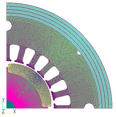
(a) XY plan view
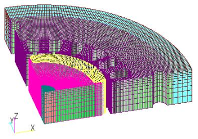
(b) Bird’s eye view
Fig.2 Analysis model (for 3D analysis)
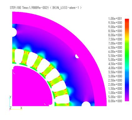
(a) Eddy current loss distribution $W_{e \perp} (W/kg)$
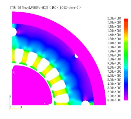
(b) Hysteresis loss distribution $W_h (W/kg)$
Fig.3 Iron loss distribution in 3-D static magnetic field analysis
by calculation method ②
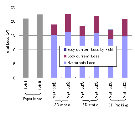
Fig.4 Iron Loss Characteristics
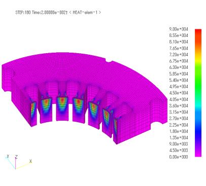
Fig.5 Eddy current loss distribution $W_{e\parallel} (W/m^3)$ in in-plane direction in 3D eddy current analysis (Packing)
In the actual verification model used in this study, both the rotor and stator are made of 50A1300 nondirectional electromagnetic steel sheets that are stacked one after another. In addition, adhesive is used to create the laminations, eliminating the effects of stress and burn-in, which are factors that degrade magnetic properties. Therefore, the results of the analysis are considered to match very well with the measurement results of the actual device. However, especially for hysteresis loss, both iron loss estimation methods ① and ② use Steinmetz’s formula, which assumes that the loss is proportional to a power of the magnetic flux density. In practice, hysteresis loss is calculated from the area of the hysteresis loop. Therefore, please be aware that it may be less accurate than the other proposed method (2), which takes it into account.
References
[1] Technical Committee for Investigation of Advanced Three-Dimensional Electromagnetic Field Analysis of Rotating Machines: “Advanced Technology for Electromagnetic Field Analysis of Rotating Machines,” Technical Report of IEEJ, No. 942 (2004)
[2] Technical Committee for Investigation of High-Precision Modeling Technology for Electromagnetic Field Analysis of Rotating Machines: “Advanced Technology for Accurate Modeling Technology”, IEEJ Technical Report, No. 1044 (2006)
How to use
Iron loss calculation is calculated as post-processing and can be done with nonlinear static and transient magnetic field analysis calculated in many steps.
(1) Since the calculation is performed as post-processing, set PRE_PROCESSING, MAKING_MATRICES, and SOLVING_EQUATION to 0 after the main calculation is executed, and set only POST_PROCESSING to 1.
(2) To calculate the iron loss per cycle, set STEP_INTERVAL in the EMSolution Handbook “9. Output Steps, Phase” to the number of steps for one cycle.
(3) Set AVERAGE to 1 in “10. Input/Output File”. This is normally used to calculate the average heat generation per cycle but is also used for iron loss calculations to output per cycle.
(4) The iron_loss file is output as an output file of iron loss distribution. Set 1 ($W/kg$) or 2 ($W/m^3$) to IRON_LOSS in “10. Input/Output File”. If you want to output heat generation, which is eddy current loss in the in-plane direction, set HEAT=1.
(5) To output iron loss for one cycle to the output file, set IRON_LOSS in the third column of “11. Printout: 11.1 Output Options” to 1 (method ①: absolute value of the maximum magnetic flux density) or 2 (method ②: magnetic flux density waveform). If HEAT=1 is set, eddy current loss in the in-plane direction can also be output.
(6) If IRON_LOSS is set to 1 (method ①), enter the frequency FREQUENCY ($Hz$) and the coefficients ALPHA, BETA, and GAMMA in the next column. All are set to 2.0.
(7) To set the iron loss coefficient, set IRON_LOSS to 1 in “16.1.1 Volume Element Properties”. Set the local coordinate COORD_ID, density MASS_DENSITY $(kg/m^3)$, eddy current loss coefficient $K_E (W/kg/T^2/Hz^2)$, and hysteresis loss coefficient $K_H (W/kg/T^2/Hz)$ to evaluate the magnetic flux density component as parameters required for iron loss calculation. Also shown is an example of PACKING and conductivity anisotropy input from a normal calculation. However, if you want to output the iron loss and magnetic flux density in the cylindrical coordinate system from the results calculated in the overall coordinate system using PACKING, you must re-set the COORD_ID of PACKING to the local cylindrical coordinate ID defined so that the z direction is in the stacking direction.
If PACKING is not used, specify a local cylindrical coordinate ID defined with the stacking direction as the z-direction in the COORD_ID parameter of the iron loss calculation.
EMSolition Version r11.2.1 New Features
From r11.2.1, eddy current loss coefficient $K_e$ and hysteresis loss coefficient $K_h$ can be set independently in the three directions to calculate iron loss. Note that the eddy current loss coefficient in the stacking direction (Z-direction) does not need to be set. This is because this component is assumed to be calculated as eddy current loss in the lamination plane ($\sigma_z= 0$) in FEM.
(8) When EMSolution is executed, eddy current loss and hysteresis loss in the stacking direction are output for each property in the output file. The eddy current loss and hysteresis loss distribution in the stacking direction are output to iron_loss as a post file. If the HEAT option is used, the in-plane eddy current loss for each property is output in the output file and its distribution is output in the post file heat in the same way.
In the FEMAP Neutral file format, the contents of iron_loss are as follows
- LOSS-elem-1 Anomalous eddy current loss (=1:$W/kg$ or =2:$W/m^3$ )
- LOSS-elem-2 Anomalous eddy current loss ($W$)
- LOSS-elem-3 Hysteresis loss (=1:$W/kg$ or =2:$W/m^3$ )
- LOSS-elem-4 Hysteresis Loss ($W$)
< Output Example >
The following shows the iron loss calculation results of the three-dimensional static magnetic field analysis.
Download
The mesh file used in the example cannot be disclosed due to geometry confidentiality. Please understand that.
Analysis Examples by Functions
Iron loss, permanent magnets and laminated iron cores
- Iron loss calculation using half-cycle periodicity
- Analysis of laminated iron cores by homogenization method and output of magnetic flux density of iron section of laminated iron core
- Analysis using nonlinear two-dimensional anisotropic magnetic properties
- Magnetization input to MAGNET by function
- Iron loss calculation by post-processing
- Evaluation of the rate of decrease from the input magnetization to the operating point and permeance coefficient of permanent magnets
- Demagnetization analysis of permanent magnets
- Analysis considering temperature dependence of magnetization properties
©2020 Science Solutions International Laboratory, Inc.
All Rights reserved.