Summary

In the finite element method, the magnetic field is usually obtained by interpolating the finite element shape function from the analysis results. EMSolution outputs the magnetic field distribution at the element center or nodal position. However, there are cases where the magnetic field at an arbitrary point is desired. In addition, the amount of data output at the element center or nodal point is large, and it may require considerable effort to find the magnetic field at the required point among them.

EMSolution has been able to obtain the magnetic field at an arbitrary spatial point by integrating the magnetic field produced by magnetization as a post-processing step.. Now, the magnetic field produced by currents (source currents and eddy currents) is also integrated. This makes it possible to obtain a magnetic field equivalent to that obtained from finite elements. This integration can be done separately for each source, and the magnetic field originating from any part of the source can also be determined.

Explanation

The magnetic field integral from the current and magnetization is performed by the equation below.

$$B(r_p) = \frac{\mu_0}{4\pi} \int_{\Omega} { (\frac{J(R)×r}{r^3}-\nabla_p(\frac {M(R) \cdot r}{r^3}) } dV$$

Here $r= r_p-R$ , $r=|r|$. $r_p$ is the coordinate of the space point to be obtained and $R$ is the coordinate of the integration point. Gaussian integral is done within each element.

A simple model (Fig. 1) illustrates this. This model simulates the IEEJ three-dimensional magnetostatic field verification model (IEEJ Technical Report (Part II) No. 286, Three-Dimensional Magnetostatic Field Numerical Calculation Techniques, December 1988). The same model is shown in “Static magnetic field analysis using ELMCUR (element current source)”.The analysis is performed with a finer mesh and the far boundary is also taken farther away. Here, the coil current is defined by “SDEFCOIL”. The magnetization is in the central core and the current is only in the coil region.

Fig. 2 shows a comparison of the magnetic field output as a nodal quantity and the magnetic field obtained by integration here. There is a slight error, but both methods are in good agreement. This error is mainly due to the boundary conditions. The far boundary condition is an electric wall with Bn=0. The boundary condition equivalently generates an error field in the computational domain. This error increases as the far boundary is moved closer, which can be used as a guide for calculation error and the location of the far boundary.

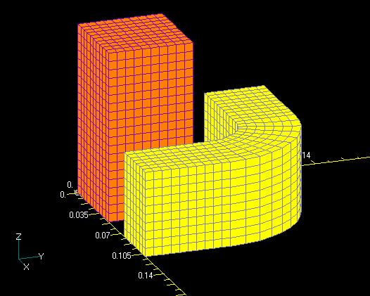
Fig.1 Analysis model

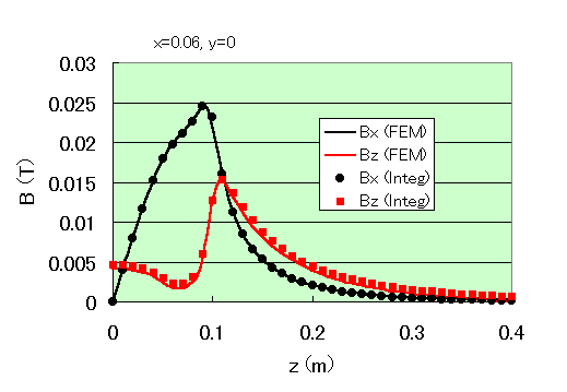
Fig.2 Magnetic field on a line at x=0.06m and y=0