Summary

EMSolution can handle ordinary rotational periodic symmetry and z-inverse periodic symmetry. Each has symmetry and anti-symmetry conditions. Here is an example for a magnetic field due to a magnet.

Explanation

Usually, the magnetic field is interpolated from the solution and shape function obtained and output at the element center or nodal point. However, it is sometimes necessary to find the magnetic field at spatial points independent of the mesh or at points outside the mesh. Interpolating these from the magnetic fields obtained at element or nodal points is a rather difficult problem. For this reason, EMSolution obtains the magnetic field by determining the magnetization in the magnetic material or magnet from the calculation results and integrating the magnetic field. Periodic conditions must be taken into account in this integration, and symmetry must be reconciled with the magnetic field calculation.

Here is an example with a simple model shown in Fig. 1. The only source of the magnetic field is the magnet, which is assumed to have periodic symmetry of 60 degrees. Assume that the magnet is magnetized (1T) in the z direction. The magnet is shifted in the z direction so that there is a difference in the type of rotational symmetry. The magnetic field on the magnetic field evaluation line shown in the figure is evaluated. The evaluation line runs through the center of the element for comparison with the magnetic field from element interpolation.

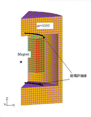
Fig.1 Analysis model

The rotational symmetry that can be used in EMSolution with this model is shown in Fig. 2. In anti-symmetry, Field quantities such as magnetic field are reversed when rotated symmetrically. Z-inverse rotational symmetry reverses the position with respect to the Z=0 plane simultaneously with the rotation. The arrows in Fig. 2 indicate the direction of magnetization. The magnetic field has the same symmetry.
In the case of rotational symmetry, the direction of the magnetic field does not change with rotation (60 degrees in this case). In the case of rotational anti-symmetry, all components of the magnetic field are reversed. In the case of z-inverse rotational symmetry, the z component is the same and the other components are reversed. In the case of z-inverse rotational anti-symmetry, the opposite is true.

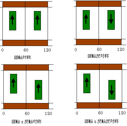
Fig.2 Rotational symmetry

Below are the results of the analysis at each symmetry. The magnetic field distribution on the magnetic field evaluation line is shown. In each figure, the $\bullet$ mark (dot) is obtained by element interpolation, and the solid line is obtained by integrating the magnetizing field. Black indicates the radial component, red the angular component, and blue the z-direction component. In reality, the magnetic field is obtained only up to 60 degrees, but it is symmetrically converted to show the magnetic field up to 120 degrees. You can see that each has the assumed symmetry. At large magnetic fields, there is a large error between those obtained from the elements and those obtained by integration. This is probably because the magnetic field gradient is so large that the shape function in the element cannot fully represent the magnetic field. For better accuracy, the mesh should be made finer. In this example, the spatial mesh on the upper side of the magnet is coarser. It is difficult to say which of the two is more accurate, but if anything, the one based on integration is considered to be more accurate.

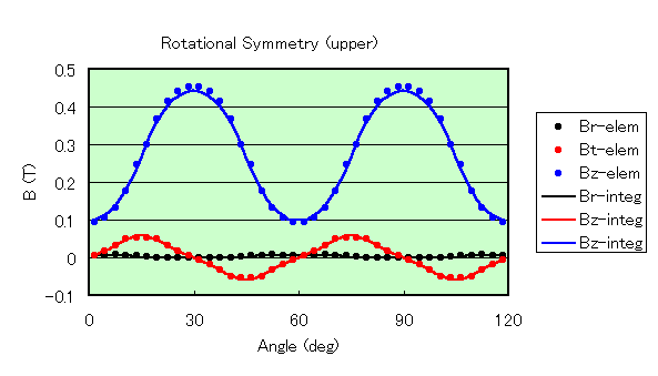
Fig.3 Rotational symmetry
(Magnetic field on the upper evaluation line)

Fig.4 Rotational symmetry
(Magnetic field on the lower evaluation line)

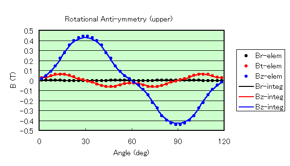
Fig.5 Rotation anti-symmetry
(Magnetic field on the upper evaluation line)

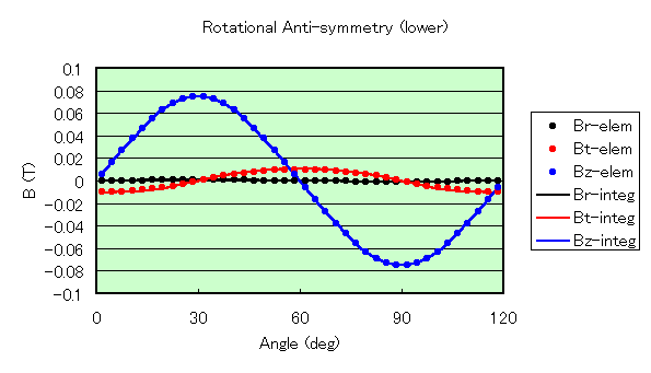
Fig.6 Rotation anti-symmetry
(Magnetic field on the lower evaluation line)

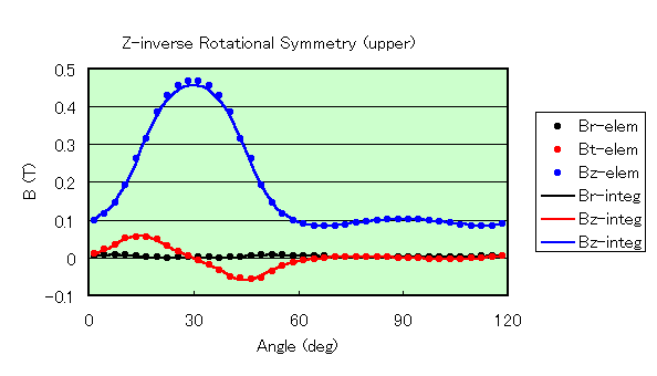
Fig.7　 Z-inverse rotational symmetry
(Magnetic field on the upper evaluation line)

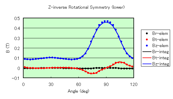
Fig.8 Z-inverse rotational symmetry
(Magnetic field on the lower evaluation line)

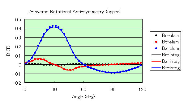
Fig.9 Z-inverse rotational anti-symmetry
(Magnetic field on the upper evaluation line)

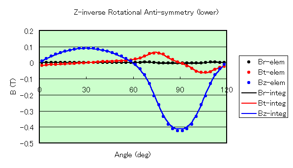
Fig.10 Z-inverse rotational anti-symmetry
(Magnetic field on the lower evaluation line)

Using rotational Z-inverse anti-symmetry, the model can be analyzed in half the time of a normal rotationally symmetric analysis. The method of integrating the magnetization field requires a longer computation time in post-processing because Gaussian integration is performed on each element. However, it is convenient because the magnetic field at any spatial point can be calculated. It is also possible to divide the magnetic field into regions and determine the contribution from only those portions. This integration can be performed for magnetic materials, magnets, and external current sources (COIL); it is also possible to integrate the magnetic fields due to source currents and eddy currents in ELMCUR and SDEFCOIL.
$\Rightarrow$ "Magnetic field by integration of magnetization and current"