Electromagnetic field analysis software

One pole modeling of a squirrel-cage induction motor

TOP >
Analysis Examples by Functions （List） >
One pole modeling of a squirrel-cage induction motor

Summary

In “Induction Motor Analysis”, we showed how to correct the conductivity of the rotor bar including the resistance of the end rings and constrain the surface integral of the total axial current to zero using SUFCUR (surface inflow current source), and in “Handling of Rotor Bars and End Rings in Two-Dimensional Analysis of Squirrel-cage Induction Motors”, we showed how to approximate the virtual resistance of the rotor bar and end rings and model the equivalent circuit including the rotor bar. The model used in these analyses is a two-pole model, but this method can also be applied to a one-pole model. However, some modifications are required for this method, which will be explained in the following. The model used in these analyses is a two-pole model, but this method can also be applied to a one-pole model. However, some modifications are required for this method, which will be explained in the following.

Explanation

Since the model in “Induction Motor Analysis” has an odd number of rotor bars (17 for two poles), a newly created model with 20 bars is used here. 20 (bars) is an appropriately determined number only for the sake of calculation, so please note that no improvement in characteristics can be expected. The model is assumed to be without skew.

Two-pole 180-degree model

This is a repeat of “Induction Motor Analysis”, but first we will show how to analyze a two-pole 180-degree model. Next, we will discuss some points to note when converting it to a single-pole 90-degree model and compare the results of the 180-degree model and the 90-degree model. The two-pole 180-degree model is shown in Fig. 1.

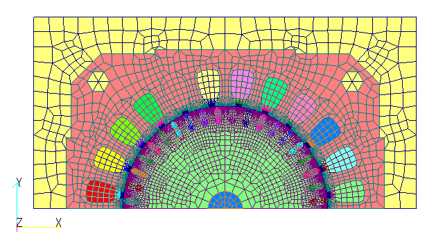
Fig.1 Analytical mesh of two-pole 180-degree model

Method (1)

First, the case in which the conductivity of the rotor bar is corrected by including the resistance of the end ring, as defined in SUFCUR, is presented. The correction method is the one described in [1] and [2]. The reason why the rotor bars are defined by SUFCUR in the analysis of the two-pole model is to set the constraint that the integral (sum) of the currents flowing in the rotor bars at two poles is zero. The current in the end ring can be expressed from the current in the rotor bar, the number of rotor slots, and the number of poles as follows [1].

$$I_r = \frac{N_2}{P \pi}I_b　　　　　(1)$$

The resistance of the end ring is calculated by converting the end ring resistance between rotor bars into the resistance per rotor bar using the following equation: [1],[2]

$$R_{r2D} = R_b + R_r \frac{N_2}{(P \pi)^2}　　　　　(2)$$

where $R_b$ is the resistance of the rotor bar and $R_r$ is the resistance of the end ring, calculated by the following equation:

$$R_b = \frac {1}{\sigma_0} \cdot \frac{I_b}{S_b}　　　　　(3)$$

$$R_r = 2 \frac{1}{\sigma_0} \cdot \frac{I_r}{S_r}　　　　　(4)$$

where $l_b$ is the length of the rotor bar, $S_b$ is the cross-sectional area of the bar, $l_r$ is the end ring circumference, $S_r$ is the cross-sectional area of the end ring, and $\sigma_0$ is the conductivity of the secondary conductor. The coefficient 2 in the expression for Rr is used to express the sum of the upper and lower values. The resistance of the end ring between the rotor bars, which is used when setting the end ring resistance in NETWORK, is expressed by the following equation, which is equation (4) divided by the number of rotor slots.

$$(R_r)_{one} = \frac{1}{\sigma_0} \cdot \frac{I_r}{S_r} \cdot \frac{1}{N_2}　　　　　(5)$$

The resistance $R_{r2D}$ per rotor bar in the two-dimensional analysis is obtained by taking the slot cross-sectional area as the rotor bar cross-sectional area and the iron core length $l$ as the length of the rotor bar ($l$ = $l=l_b$ when there is no skew), so the effective conductivity $\sigma_{eff}$ is expressed by:

$$R_{r2D} = \frac{1}{\sigma_{eff}} \cdot \frac{l}{S_b}　　　　　(6)$$

Therefore, the effective conductivity $\sigma_{eff}$ can be obtained from the following equation.

$$\sigma_{eff} = \frac{l}{R_{r2D}S_b} = \frac{R_b}{R_{r2D}} \sigma_0　　　　　(7)$$

The effective conductivity of the model with two-poles and 20 rotor bars used in this study is 1.0598 × 107S/m. Here, the rotor bar cross section is assumed to be $1.41 \times 10^{-5}m^2$, which is the elemental cross section, the end ring cross section is $1.781 \times 10^{-5}m^2$ based on the dimensions in Reference [2], the end ring circumference is $0.19m$, and the conductivity of the secondary conductor, aluminum, is $2.9841 \times 10^7 S/m$. This value is larger than the original model’s value of $1.02 \times 10^7 S/m$, but this is thought to be due to the fact that the original model corrects for changes in resistance due to temperature rise. In this calculation, only the dimensions and catalog values are used.

Method (2)

The following is a case in which NETWORK simulates an end ring as a resistance. The conductivity of the rotor bar is that of aluminum, and the resistance of the end ring is 8.9394 $\mu \Omega$, calculated as the end ring resistance between the rotor bars from formula (5) (the original model value is 10.50 $\mu \Omega$). Since this is a 1/2 model, REGION_FACTOR=2 Is set, and the end ring resistance is multiplied by 2.

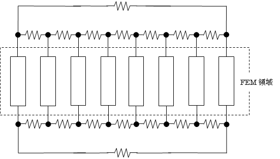
Fig.2 Equivalent circuit of rotor bars and end rings
(Two-pole 180-degree model)

Fig.3 Current variation in stator primary winding
(Two-pole 180-degree model)

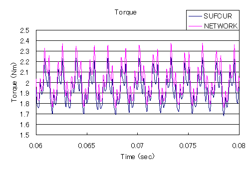
Fig.4 Torque change
(Two-pole 180-degree model)

One-pole 90-degree model

Next, one-pole 90-degree model is shown in Fig. 5. We apply methods (1) SUFCUR and (2) NETWORK to the 90-degree model as well.

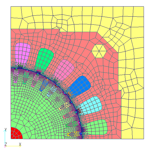
Fig.5 Analytical mesh of one-pole 90 degree model

Method (1)

When applying (1) SUFCUR to the 90-degree model, it is necessary to change the settings slightly. In the two-pole model, the current loops between the poles, so that, for example, current flowing in the +Z direction at one pole will enter the -Z direction at the other pole. In contrast, in the one-pole model, the current does not loop between the poles, but rather loops in the axial direction, flowing out in the +Z or -Z direction. Therefore, a constraint is needed to make the sum of the axial currents zero. Therefore, by connecting SUFCUR to a constant voltage source with zero voltage, the constraint can be imposed and the analysis can be performed. Since this is a two-dimensional analysis, if the boundary condition $B_n$=0 is set on the top and bottom surfaces, the current will flow according to the conductivity, the current will be conserved, and the sum of the currents on the top and bottom surfaces will be zero. Therefore, the rotor bars can be defined as conductors with corrected conductivity without using SUFCUR.

Method (2)

Consider applying NETWORK to a single pole. The current flowing in the rotor bar and end rings for one cycle corresponds to the current for two poles, as shown in Fig. 6. Focusing on the direction of current flow in the end ring, we see that we can represent it using one-pole model with the upper and lower wires crossed. Therefore, by connecting the wires as shown in Fig. 7, it is possible to model the current as one-pole model. This method can be applied not only to squirrel-cage induction machines, but also to generators and large field-wound synchronous machines with a cage (short-circuit ring). In this case also, care must be taken with the REGION_FACTOR setting, and the resistance of the end ring must be multiplied by REGION_FACTOR. Since this is a 1/4 model, REGION_FACTOR=4 and the resistance of the end ring is multiplied by 4.

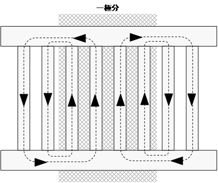
Fig.6 Currents in rotor bars and end rings for two-pole (one pole pair) model

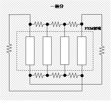
Fig.7 Equivalent circuit of rotor bars and end rings (One pole 90-degree model)

As with the 180-degree model, for the 90-degree model, Fig. 8 shows the current variation in the primary stator winding and Fig. 9 shows the torque variation at slip S = 0.25. As with the two-pole model, good agreement is observed for methods (1) SUFCUR and (2) NETWORK. The difference from the 180-degree model is less than 0.002%, which is not surprising, but shows very good agreement. In this way, the induction machine can be analyzed with the one-pole model. If there is one pole periodicity, the one-pole model is advantageous from a computational point of view. The choice between SUFCUR and NETWORK will depend on the extent to which the analysis is to be performed, so please select and use accordingly.

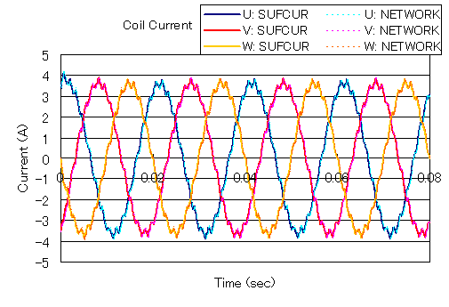
Fig.8 Current variation in stator primary winding
(One-pole 90-degree model)

Fig.9 Torque variation
(One-pole 90-degree model)

References

akeuchi: “Electric Design Science”, Ohmsha Co.
Electromagnetic Field Analysis Techniques for Virtual Engineering of Rotating Machines,” IEEJ Technical Report No. 776 (2000)

Download

Two-pole 180-degree model

SUFCUR Model

・ input_180deg_SUFCUR_S0_25.ems ：Transient analysis with slip 0.25
・ inputAC_180deg_SUFCUR_S0_25.ems ：AC analysis with slip 0.25
・ pre_geom2D.neu ：Stator mesh data
・ rotor_mesh2D.neu ：Rotor mesh data