Summary

Using a two-dimensional analysis of an induction motor as an example, the new capabilities of EMSolution will be explained.

Explanation

The following two new features have been added to EMSolution:

1. The sliding method can now be used in AC steady-state analysis.

The sliding method of joining fixed and movable sections has been limited to magnetostatic and transient analyses, but it can now also be used for AC steady-state analysis. This allows AC steady-state, static magnetic field, and transient analyses to be handled in a unified manner on the same mesh. In addition, by effectively changing the rotation frequencies of the fixed and movable sections, slip effects can be included.

2. Transient analysis can now be performed using the result of the AC analysis as initial values.

To obtain a nonlinear steady state, transient analysis must be performed until the steady state is reached. However, when the time constant of the system is large, transient conditions may persist for a long time and require many steps of analysis. Starting from zero initial value may require a large number of steps and excessive calculation time. In this case, if the results of an AC steady-state analysis (currently limited to linear analysis) are used as the initial values, the steady state can be reached relatively quickly. The results shown here are from a two-dimensional analysis and do not include the effect of the skew of the rotor bars, but, if necessary, a three-dimensional analysis with skew can be performed as well.

Fig. 1 shows the mesh model used in the analysis, and Fig. 2 is an enlarged version of it. The gap region is divided into four layers, with a sliding surface at the center plane. The model is rotationally symmetric by 180 degrees, and half of the entire model is analyzed. The three phase stator windings are assumed to be Y-connected and voltage driven. The rotor bar is also given an equivalent electrical conductivity taking into account the end rings, and the total current in the z-direction is set to zero by using EMSolution’s SUFCUR.

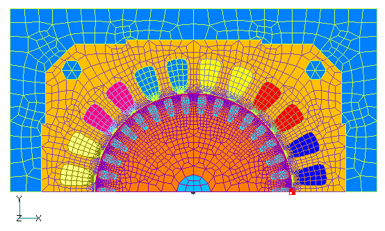
Fig.1 2D mesh model of induction generator

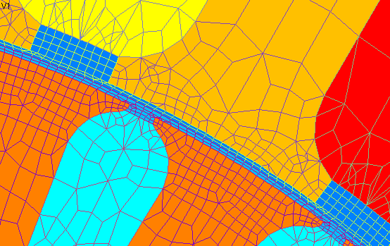
Fig.2 Partial detail of 2D mesh model of induction generator
The air gap region is divided into four layers.
The sliding surface is placed at the center of the slide.

Fig. 3 shows the analytical results of the current variation in the primary stator winding when the rotor is not in motion (slip S=1). Negative times show the results of the AC steady-state analysis, while positive times show the results of the analysis using that as the initial value. The AC steady-state analysis is performed as a linear calculation by giving appropriate permeability. Although small oscillations are observed at the beginning of the transient analysis, it soon reaches a steady state and transients are no longer observed. In this analysis, starting from zero initial value, about 10 cycles are required to reach steady state. In Fig. 3, a nearly steady solution is obtained in the second period. Fig. 4 shows the rotational torque acting on the rotor, which also reaches near-stationarity in the second cycle. From Figs. 3 and 4, it can be seen that the primary winding current and average torque can be evaluated by AC analysis.

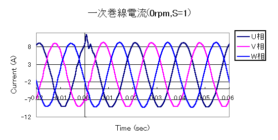
Fig.3 Current variation in the primary stator winding in case of no rotor rotation (slip S=1)

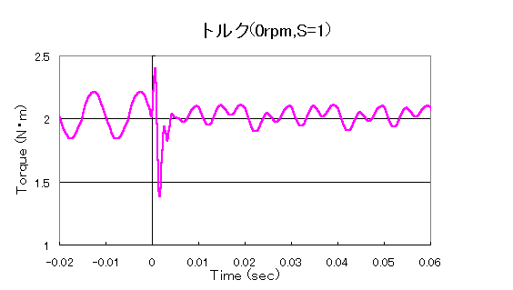
Fig.4 Torque acting on the rotor (half) in case of no rotor rotation (slip S = 1)

Figs. 5 and 6 show the results for a rotor speed of 1125 rpm and slip S = 0.25. In this case, the AC steady-state analysis shows a slightly lower primary winding current and higher average torque, but still reaches steady state in the second cycle of transient analysis. The result of the AC steady-state analysis depends on the input magnetic material linear permeability, which in this example does not seem to affect the transient analysis very much.

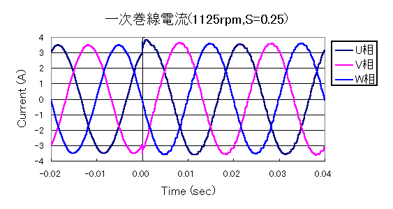
Fig.5 Current variation in stator primary winding in case of RPM 1125ppm with slip S=0.25

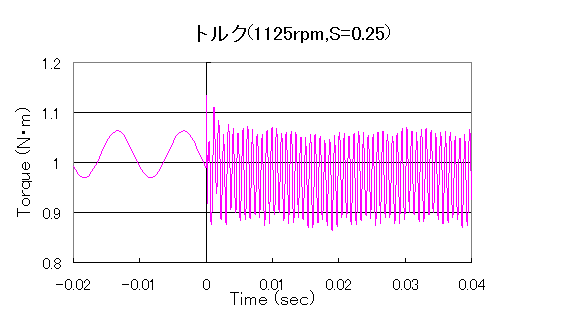
Fig.6 Torque acting on the rotor (half) in case of RPM 1125ppm with slip S=0.25

Figs. 7 and 8 show the magnetic flux density intensity and magnetic flux distribution in iron material. The magnetic flux is the amount of magnetic flux passing through the specified width in the z-direction (DELTA_Z=42mm). The magnetic field is oriented in the direction of the isomagnetic flux lines. It can be seen that the magnetic flux lines are normally continuous across the slide plane. Fig. 9 shows part of the flux density arrow diagram for the same case. Fig. 10 shows the current density variation in the primary winding and rotor bar. Although it may be difficult to understand because only one cycle is shown, it can be seen that the rotor rotates with a slip S = 0.25 slower than the rotation of the current distribution in the primary winding, and that the current in the rotor bar rotates at the same speed with almost the opposite phase of the primary current.

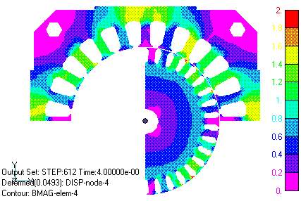
Fig.7 Magnetic flux density intensity distribution
(S=0.25, 0.04sec), unit $T$

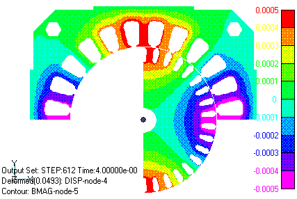
Fig.8 Magnetic flux distribution
(S=0.25, 0.04sec), unit $Wb$

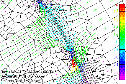
Fig.9 Magnetic flux density arrow diagram
(S=0.25, 0.04sec), unit $T$

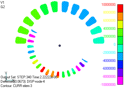
Fig. 10 Rotor bar current density of primary winding
(S=0.25, 0.02-0.04sec), unit $A/m^2$

References

Reference [1] was used as a reference in the development of this analysis method.

We would also like to express our gratitude to Prof. Katsumi Yamazaki of Chiba Institute of Technology for his kindness and guidance, and we hereby express our thanks to him.

[1] Yamazaki, Shimpuku (Chiba Institute of Technology) "Characteristic Analysis of Induction Motor Considering Neutral Point Potential Fluctuation," IEEJ Joint Study Group on Stationary and Rotating Machines, SA-99-23,RM-9