Summary

In EMSolution, we have provided various functions to handle the magnetic properties of magnetic materials. For example, “Analysis of Nonlinear Two-Dimensional Anisotropic Magnetic Properties” shows an analysis method that takes into account direction-dependent magnetic properties, such as anisotropic electromagnetic steel sheets. In addition, the paper “Analysis of laminated iron core by homogenization method” shows how to approximate and calculate objects that are not homogeneous at the microscopic level, such as laminated steel sheets, as homogeneous materials. Furthermore, “Calculation of Iron Loss by Post-Processing” shows a method for evaluating iron loss.
In recent years, it is required to calculate iron loss as accurately as possible when developing low-loss electric devices. In the iron loss evaluation method by post-processing described above, the iron loss can be easily calculated by approximating the magnetic property by initial magnetization curve, but for more accurate calculation, it is important to use an analysis method that directly considers the effect of hysteresis of magnetic materials. In this situation, we have developed a hysteresis analysis function that applies the hysteresis model, the Play model, to EMSolution.

Explanation

1. Play model

Although many modeling approaches have been proposed to express hysteresis magnetic characteristics, we have adopted the Play model, which has recently attracted much attention. The Play model is represented by a simple operator called hysteron, which delays the phase of the output relative to the input. Fig. 1 shows the operating characteristics of the play hysteron. The hysteron is represented by a simple equation as in equation (1), which is equivalent to the behavior of a two-cart model as shown in Fig. 2. In equation (1), $\zeta$ is the hysteron width, $B$ is the magnetic flux density, $p$ is the hysteron, and $p_0$ represents the past hysteron. The play model is obtained by preparing hysterons of various $\zeta$, acting on each hysteron with a function called the shape function, and taking the sum of all the hysterons.

$$p_{\zeta}(B) = B-\frac{\zeta(B-p^{0})}{max(|B-p^{0}_{\zeta}|)}$$

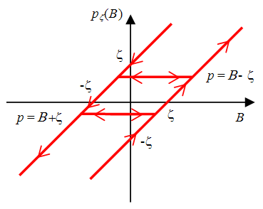
Fig.1 Playhisterone

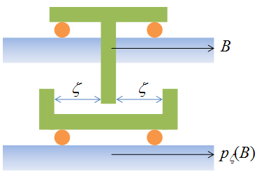
Fig.2 Bogie model

Fig. 3 shows the hysteresis curve of an electromagnetic steel sheet equivalent to 50A470, expressed using the Play model. Since the Play model is a mathematical model based on measured data, it requires measured data in a specified format. Since the accuracy of the measured data may affect the accuracy of the magnetic field analysis and the nonlinear convergence characteristics, it is necessary to devise ways to improve the accuracy of the data. Since the play model calculation is performed using the shape function derived from the measured data, the shape function has to be identified from the measured data prior to the magnetic field calculation. We will show how to do this in the next issue.

Since the Play model is a model that expresses DC magnetic properties, and the shape function is identified from DC magnetization properties that do not include the effects of eddy currents, in the analysis model with a fluctuating magnetic field, the conductivity is set as input data for EMSolution as before, and the eddy current field is solved.

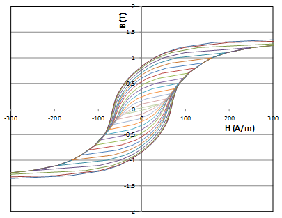
Fig.3 Hysteresis curve represented by the play model

2. Hysteresis analysis using ring samples

Hysteresis analysis is performed using the ring sample shown in Fig. 4. The analysis is performed with the mesh data, pre_geom2D.NEU, and the analysis condition file input. The shape function file required for the play model analysis is shape.
If eddy currents in the sample are neglected, the analysis becomes a two-dimensional static analysis, but the component of the magnetic field in the radial direction of the sample is small, so the model is in fact a one-dimensional model. Since there are no voids in the ring sample and no magnetic poles appear, it can be said to be an analysis model in which the effects of hysteresis are noticeable. As initial conditions, the ring sample is assumed to be demagnetized and a sinusoidal current of 0.05 $Hz$ and a maximum of 5 $AT$ is applied to the coil.

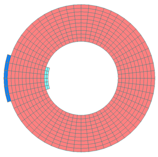
Fig.4 Ring sample

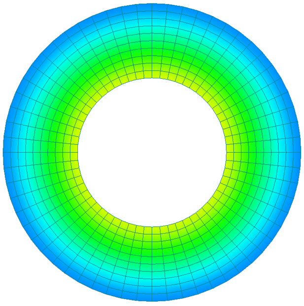
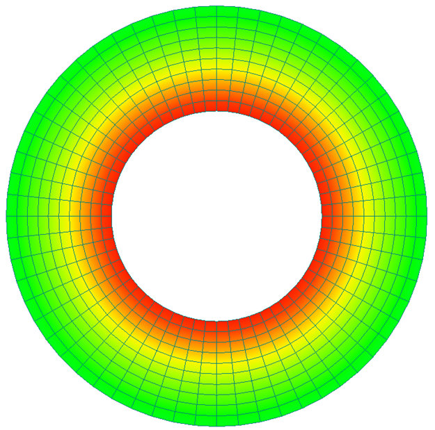
Fig. 5 shows the temporal variation of the magnetic flux density distribution. As can be seen from the figure, the magnitude of the current at (a) 2.5s when the current increases and (c) 7.5s when the current decreases are equal, but the magnetic flux density distribution is different because the ring is magnetized. Fig. 6 shows the time variation of the current flowing in the coil and the amount of magnetic flux linkage to the coil. It can be seen that the phase of the magnetic flux quantity lags behind the current, which is qualitatively correct.

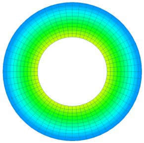
(a)　2.5s

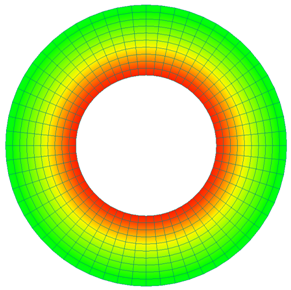
(b)　5s

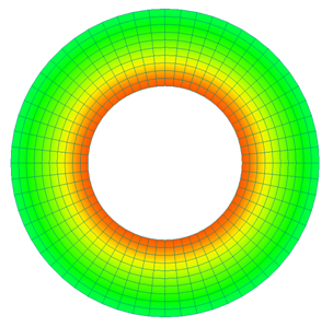
(c)　7.5s

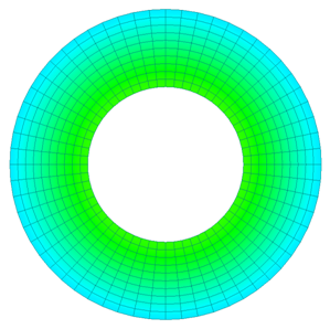
(d)　10s

Fig.5 Magnetic flux density distribution

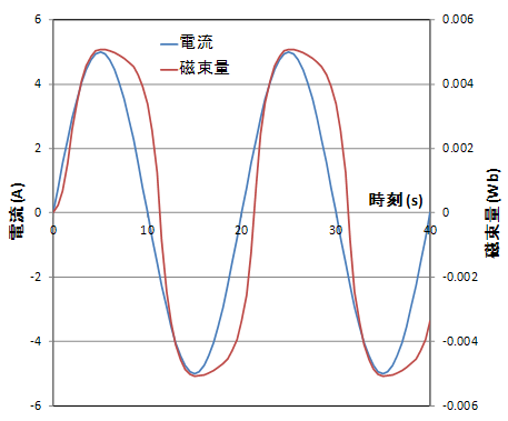
Fig.6 Time variation of current and magnetic flux

Please refer to the references for further explanation. However, the hysteresis material and other factors are different from those in the text.

3. Hysteresis loss distribution

Similar to the “Iron Loss Calculation by Post-processing”, the hysteresis loss distribution of a hysteresis analysis using Play model can be output as post data. The hysteresis loss distribution for the ring sample model described above is shown in Fig. 7(a). The iron loss is evaluated not in the first period starting from the initial state of no-excitation, but in the period after the second period when a steady state is reached. Fig.7(b) shows the hysteresis loss distribution calculated in “Iron loss calculation by post-processing” (calculation method ②). Fig. 8 graphs the results of each calculation method as distribution values in the radial direction. In the post-processing iron loss calculation, the hysteresis loss changes in proportion to the square of the magnetic flux density, but in the Play model calculation, the loss is calculated according to the hysteresis characteristics actually measured. The hysteresis characteristics used in the Play model calculations are based on actual measurements, but the iron loss coefficients in the post-processing were obtained from the manufacturer’s catalogs.

(a) Play model calculation

(b) Post-processing

Fig.7 Hysteresis Loss Distribution Unit[$W/m^3$]

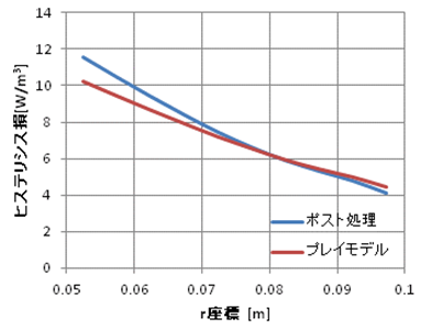
Fig.8 Comparison of hysteresis loss distribution between Play model and post-proseccing