Electromagnetic field analysis software

Electromagnetic field analysis software
Hysteresis loss calculation by Play model post-processing
- TOP >
- Analysis Examples by Functions (List) >
- Hysteresis loss calculation by Play model post-processing
Summary
EMSolution can perform “hysteresis analysis using the Play model” for nonlinear problems involving magnetic materials. We have now added a new feature to calculate hysteresis loss using the Play model in post-processing based on the result obtained by a conventional magnetic field analysis using initial magnetization properties without hysteresis.
Explanation
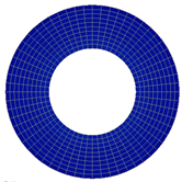
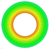
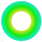
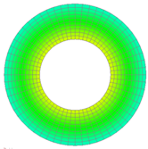
First, a magnetic field analysis using the initial magnetization characteristics is performed using the model in “Hysteresis analysis with Play model”. The magnetization characteristics used here are shown in Fig. 1. The analysis results are shown in Fig.2 and Fig.3. The results of hysteresis analysis are also shown for reference.
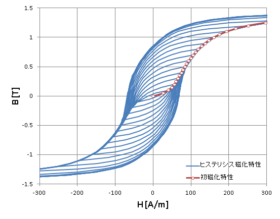
Fig.1 Magnetization characteristics
2.5s
5.0s
7.5s

10.0s
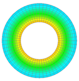
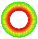
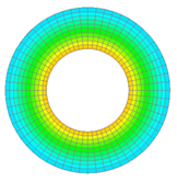
(a) Conventional analysis based on initial magnetization characteristics

2.5s
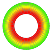
5.0s
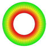
7.5s
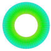
10.0s
(b) Hysteresis analysis
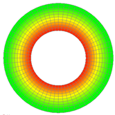
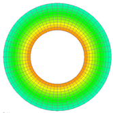
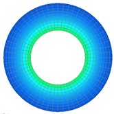
Fig.2 Magnetic flux density distribution
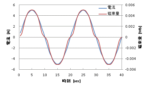
(a) Conventional analysis based on initial magnetization characteristics
(b) Hysteresis analysis
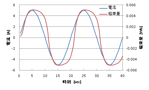
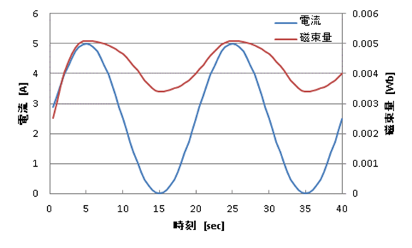
Fig.3 Time variation of current and magnetic flux
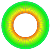
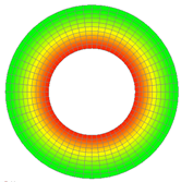
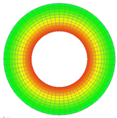
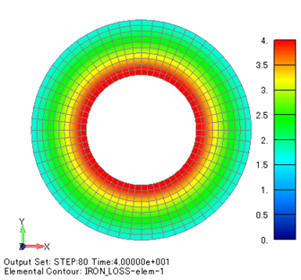
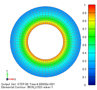
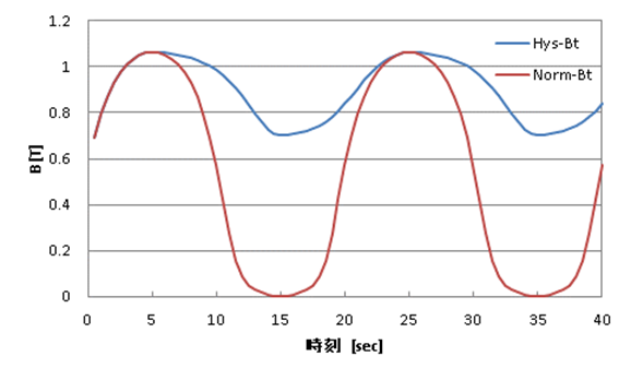
Using the analysis data from the initial magnetization characteristics, the play model calculation can be performed in post-processing to calculate the hysteresis loss. Fig. 4(a) shows the hysteresis loss distribution. The results of each calculation method are graphed as distribution values in the radial direction as shown in Fig. 5. Hys-Loss3 and Norm-Loss3 are the distributions when hysteresis loss is calculated by the Play model calculation in the hysteresis and conventional analyses, respectively (iron loss output option IRON_LOSS(11) = 3). Hys-Loss2 and Norm-Loss2 are the distributions when hysteresis loss is obtained from the hysteresis loss coefficient (derived from the manufacturer’s catalog) (Iron loss output option IRON_LOSS(11) = 2). The results of the hysteresis analysis and the post-processing Play model calculations are almost identical. Fig. 6 shows the circumferential magnetic flux density (B_t) variation of the innermost element for both hysteresis and conventional analysis. The changes in flux density are different, but the amplitudes are almost the same. Since the magnetic field variation in this model is an alternating magnetic field, the behavior of the play model in BH space shows the same history as shown in Fig. 7, and the hysteresis loss is almost the same.
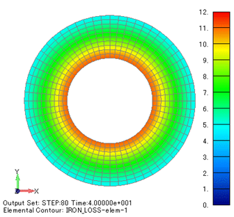
(a) Conventional analysis
+ post-processing Play model

(b) Hysteresis analysis
Fig.4 Hysteresis Loss Distribution Unit [$W/m^3$]
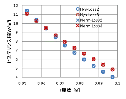
Fig.5 Comparison of hysteresis loss distribution
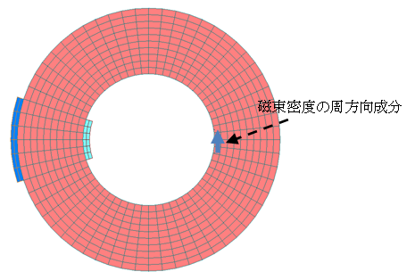
(a) Evaluation Point
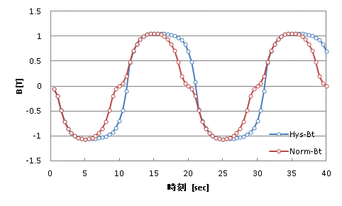
Hys-Bt: Bt in hysteresis analysis, Norm-Bt: Bt in conventional analysis
(b) Magnetic flux density at evaluation point
Fig.6 Time variation of magnetic flux density
(a) Conventional analysis
+ post-processing Play model
(b) Hysteresis analysis
Fig.7 Hysteresis Loss Distribution Unit [$W/m^3$]
Fig. 8 shows the change in the amount of magnetic flux when applying a bias DC magnetization current.
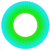
Fig. 9 shows the change in the magnetic flux density distribution.
Fig. 10 shows the hysteresis loss obtained by post-processing the Play model calculation using the results of the conventional analysis and the hysteresis loss obtained by the hysteresis analysis, respectively.
The conventional analysis results in higher hysteresis loss due to the larger magnetic field amplitude.
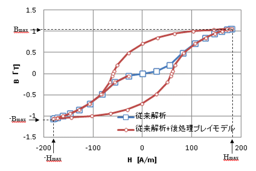
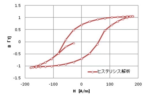
The circumferential flux density variation of the innermost element is shown in Fig. 11, and the BH behavior is shown in Fig. 12.
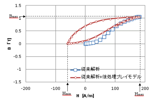
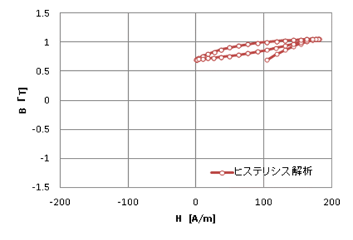
As can be seen from Fig. 12, in the initial magnetization curve, $B$ returns from $B_{max}$ to $0$ when changing from $H = H_{max}$ to $0$.
In the hysteresis analysis, however, $B$ does not go to $0$ even when changing from $H = H_{max}$ to $0$.
The magnetic field changes between $H = 0$ and $H = H_{max}$ in the hysteresis magnetization characteristic.
If the results of the conventional analysis are post-processed in the Play model, the behavior of $B$ changes from $B_{max}$ to $0$, so $H_{min}$ is less than $0$ in the hysteresis magnetization characteristic.
In the case without bias DC magnetization as shown in Fig. 7, the value of $B$ corresponding to $H = H_{max}$ ($B_{max}$ ) and the value of B when B changes from there to $H = -H_{max}$ ($-B_{max}$) are the same for the initial magnetization property and the hysteresis magnetization property, so that the hysteresis loss is also calculated to approximately the same value.
Thus, if the amplitude of the magnetic flux density is almost the same, a similar hysteresis loss can be obtained by post-processing the Play model calculation using the results of the conventional analysis, but if not, the error can be large.
The hysteresis loss calculations will also differ in cases where the model generates rotating magnetic fields that are rarely seen in the present model.
If it is necessary to calculate the time variation of the magnetic flux of a ring sample in a way that takes into account the effect of hysteresis, a hysteresis analysis should be performed.
For example, in the case of the same ring sample described above but driven by voltage, hysteresis analysis is expected to give more realistic results.
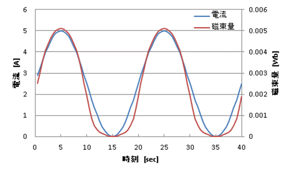
(a) Conventional analysis based on initial magnetization characteristics
(b) Hysteresis analysis
Fig.8 Temporal variation of current and magnetic flux

2.5s
5.0s
7.5s
10.0s
12.5s

15.0s

17.5s

20.0s
( a ) Conventional analysis based on initial magnetization characteristics
2.5s
5.0s
7.5s
10.0s
12.5s
15.0s
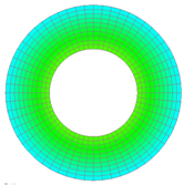
17.5s
20.0s
( b ) Hysteresis analysis
Fig.9 Magnetic flux density distribution
(a) Conventional analysis
+ post-processing Play model
(b) Hysteresis analysis
Fig.10 Hysteresis loss distribution Unit [$ W/m^3 $]
Hys-Bt: Bt in hysteresis analysis,
Norm-Bt: Bt in conventional analysis
Fig.11 Time variation of magnetic flux density
(a) Comparison between conventional analysis and Play model
post-processing
(b) Hysteresis analysis
Fig.12 H-B Operation
Table 1 summarizes the above analysis conditions and results.
Table1 Analysis conditions and hysteresis loss
| conventional analysis | Hysteresis analysis | conventional analysis | Hysteresis analysis | |
|---|---|---|---|---|
| Current Amplitude [ $A$ ] | 5 | 5 | 2.5 | 2.5 |
| Bias DC magnetization [ $A$ ] | 0 | 0 | 2.5 | 2.5 |
| Magnetic field amplitude [ $Wb$ ]. | 0.005098 | 0.005096 | 0.002549 | 0.001291 |
| Hysteresis loss A [ $J/m^3$ ]. | 139.0 | 138.8 | 34.7 | 3.8 |
| Hysteresis loss B [ $J/m^3$ ]. | 147.8 | 147.7 | 53.6 | 9.0 |
Conventional analysis: Conventional magnetic field analysis based on initial magnetization characteristics
Hysteresis Analysis: Hysteresis Analysis by Play model
Hysteresis Loss A: Post-processing using hysteresis loss coefficients
His Loss B: Play model calculation
How to use
Please refer to the model used to explain hysteresis analysis for how to calculate hysteresis loss when hysteresis analysis is performed. This section describes how to perform a conventional analysis using the initial magnetization curve and apply the Play model in post-processing to calculate hysteresis loss.
First, we will set up the post-processing.
Since this is post-processing, the asymmetric matrix solver is not used, but MATRIX_ASYMMETRICITY(3) = 1, as in the Play model analysis.
To calculate the iron loss for one cycle, set STEP_INTERVAL in the EMSolution Handbook “9. Output Steps, Phase” to the number of steps for one cycle.
Set AVERAGE in the “10. Input/output file” to 1 and calculate the total loss for each cycle.
Set IRON_LOSS(11) (Handbook 11.1 output option) to 3. And specify 2 for the output unit IRON_LOSS(10) (Handbook 10.2 Output File). Note that if you specify 1, nothing will be output in the post data.
Set ANISOTROPY = 5 in the settings for the magnetic material to which the Play model post-processing is applied. For two-dimensional Play model, enter the coordinate system COORDINATE_ID, the specific magnetic permeability MYU_Z in the Z direction, the calculated width of the magnetic flux density DB_CAL ( $T$ ), and the material identification number PLAY_ID of shape, in the next line. DB_FACTOR has no meaning in post-processing and does not need to be entered. Place the shape function file shape of the play model in the analysis folder and perform post-processing.
In the case of hysteresis analysis with a restart, the post Play model calculation refers to the hysteresis history before the restart, but in the case of conventional analysis using the initial magnetization curve, when the restart is performed, the post Play model calculation assumes that the initial state is unmagnetized.
Download
Ring model
・ Conventional analysis : input_norm
・ Post-processing by iron loss coefficient : input_norm_iron_loss2
・ Post-processing by Play model : input_norm_post_playmodel_iron_loss3
・ Mesh data : pre_geom2D.NEU
・ Shape function file of the play model : shape
* If you are interested in a trial, please contact us “here”.
Analysis Examples by Functions
Hysteresis analysis
©2020 Science Solutions International Laboratory, Inc.
All Rights reserved.