Summary

An example of magnetostatic analysis of an infinite length solenoid coil is shown. Originally, the analysis is two-dimensional, but since the current flows in the xy-plane, a three-dimensional analysis is performed using a single layer of mesh.

Explanation

An example of magnetostatic analysis of an infinite length solenoid coil is shown below. The analysis model mesh is shown in Fig. 1. A two-dimensional mesh is created and extruded 0.01m in the z direction to create a solid element. Fig.2 shows the boundary conditions for this analysis. The upper and lower surfaces (z=0,z=0.01) impose the condition $H_t=0$. The symmetry plane (x=0,y=0) is set to $B_n=0$, and the boundary condition of $H_t=0$ is imposed on the outer surface of the coil (r=1.0). At the outer surface of the coil, the magnetic field is zero, but if we impose the condition Bn=0, the magnetic vector potential in that plane will be zero and the outer integral will also be zero, thus imposing the condition that the amount of magnetic flux inside is zero.
The next step is to define the current source, and for such an irregular mesh, the definition by SDEFCOIL (surface-defined currents) is more suitable. Fig. 3 shows the defined coil surface mesh. Each of the four surfaces surrounding the coil is defined by a different physical property. Fig. 4 shows the coil current density distribution with this definition. Figures 5 and 6 show the flux density distribution computed by EMSolution. The expected magnetic field is obtained. Fig. 7 shows a comparison of the magnetic field values for all elements with the theoretical values. Although the overall agreement is good, the errors are quite large. If more accuracy is required, it is necessary to use a finer mesh or a smaller distortion of the element geometry.
An analysis of an axisymmetric shape such as the one performed here can also be analyzed with axisymmetric two-dimensional calculations. Even if it is not axisymmetrical, the analysis in this example is still applicable.

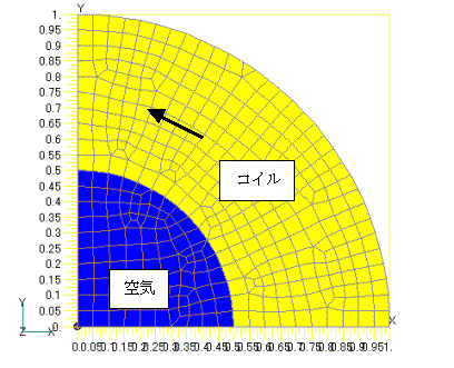
Fig.1 Analysis model

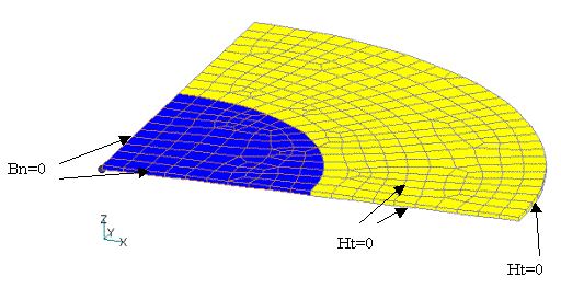
Fig.2 Boundary conditions
(Ht=0 for top and bottom surfaces, Bn=0 for symmetry surfaces, and Ht=0 for outer surface of coil)

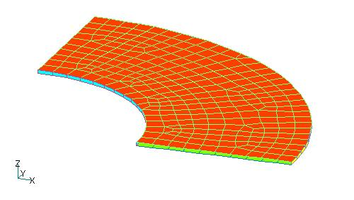
Fig.3 Coil Definition by SDEFCOIL Coil
The coil is defined in 4 planes surrounding the coil

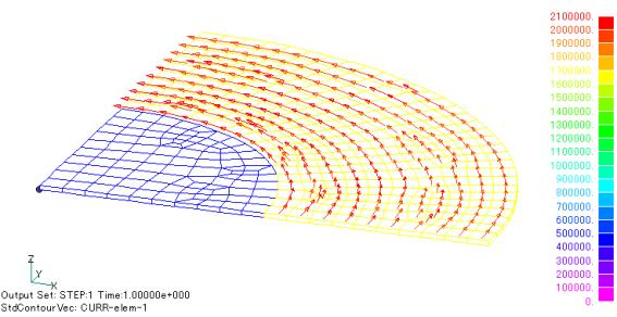
Fig.4 Current density distribution (unit $A/m^2$)

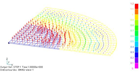
Fig.5 Magnetic flux density distribution (unit T)

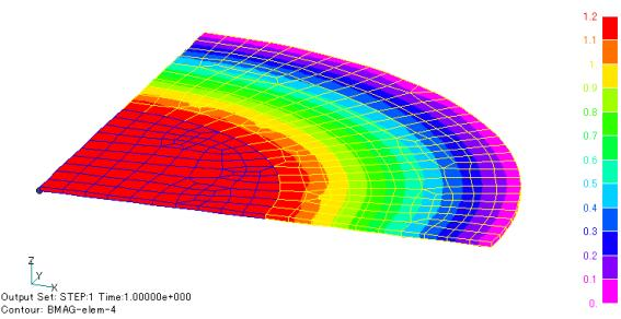
Fig.6 Magnetic flux density intensity distribution (unit T)

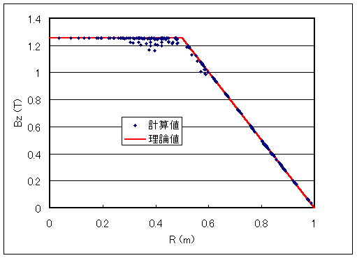
Fig.7 Comparison of calculated (element amount) and theoretical values of magnetic flux density Z component