Summary

EMSolution can perform transient analysis using the restart function, with the results of the static magnetic field analysis as the initial state and a new constant-current or constant-voltage power supply connected to the coil. As shown in "Analysis of a coil with a constant voltage power supply connected", the results of the previous transient analysis can be used as the initial state and the analysis can be continued. In this case, the constant-current power supply can be changed to a constant-voltage power supply. It is also possible to restart the analysis by changing the constant-voltage power supply to the constant-current power supply, and vice versa. This allows analysis that includes various switching mechanisms. Here is a simple example where a constant-current power supply and a constant-voltage power supply are used alternately in time.

Explanation

As an example, we will use the same model used in "Analysis of a coil with a constant voltage power supply connected". That is, we use a square coil model with a linear magnetic block in the center, as used in " Static magnetic field analysis using ELMCUR (element current source)". First, a constant-current power supply is used to linearly ramp up the current from 0A to 1A in 0.1 seconds for a 3000T coil. Then, with the power supply as a constant-voltage power source, the current is dropped with the voltage at 0 V (short-circuit condition) for 0.1 sec. At time 0.2 sec, the power supply is again set to constant current and the same cycle is repeated.

The results are shown in Fig. 1. In the constant current phase between 0 and 0.1 sec and between 0.2 and 0.3 sec, the current is the input and the voltage is obtained; in the constant voltage phase between 0.1 and 0.2 sec and between 0.3 and 0.4 sec, the opposite is true. This is in good agreement with what is obtained from the circuit calculation as shown in the analysis of the coil with the constant voltage supply connected (not shown in the figure).

In this analysis, EMSolution is run for each of the four phases. The input data are input.1, input.2, input.3, and input.4 of the sample data. No pre_processing is required after the second run. Please note that each execution starts with step number 1. The mesh files pre_geom2D.neu and 2D_to_3D are the same as used in " Static magnetic field analysis using ELMCUR (element current source)". For constant-voltage power supplies, enter the current value from the previous run as the initial current value. For constant-current supplies, no initial voltage value is required; the calculation is performed in 11 steps in order to produce a time derivative of 10 steps. For each, the initial condition is the state of the previously executed 10th step. The output solutions file is renamed old_solutions and used for the next run.

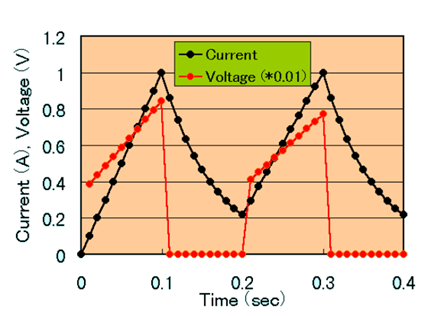
Fig.1　Time variation of coil current and voltage